Confused by complex code? Let our AI-powered Code Explainer demystify it for you. Try it out!
Many steps are involved in the data science pipeline, going from raw data to building an optimized machine learning model for the given task. However, data processing is the step that requires the most effort and time, and which has a direct influence and impact on the performance of the models later on.
In this article, we will focus on how to apply some feature selection to our dataset, which represents a core aspect of the data preprocessing phase. But before diving into coding and implementing the different techniques used for these tasks, let us first define what we mean by feature selection.
Feature selection is the process of choosing a subset of features from the dataset that contributes the most to the performance of the model, and this without applying any type of transformation on it.
The dataset we will use is the Heart Disease Prediction dataset from Kaggle and you can directly work on that using the Kaggle Kernel VM, or you can download it to your local machine.
The following is the command for installing the required libraries for this tutorial:
$ pip3 install numpy pandas matplotlib sklearnPreprocessing
We will first load our dataset into a dataframe format using pandas. It is composed of 13 features plus the label and there are 270 rows.
import numpy as np
import pandas as pd
import matplotlib.pyplot as plt
from sklearn.model_selection import train_test_split
from sklearn.preprocessing import MinMaxScaler
from sklearn.feature_selection import SelectKBest,chi2,RFE
from sklearn.ensemble import RandomForestClassifier

df = pd.read_csv("data/Heart_Disease_Prediction.csv")
print(df.shape)

df.head(5)
The above code imports the necessary libraries and reads the dataset CSV file from data folder, to follow along, you need to create data folder as well, you can change the path to the location of the dataset file in your machine.
Below is the output:
(270, 14)
From here, we can clearly observe that there are no null values, so we can directly start working on our data frame without performing some null values cleaning.
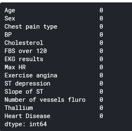
We will store the label column into a separate variable and drop it entirely (hence, the use of inplace=True) from the dataframe. This step is important when we will be dividing our dataset into training and testing in addition to when we will be fitting them to our model.
label = df["Heart Disease"]
df.drop("Heart Disease", axis=1, inplace=True)
It is important to always check how imbalanced our dataset might be since a big imbalance ratio between the minority and majority classes will negatively affect the model in a sense that it will predict only the majority class naively. For our case, however, the imbalance ratio is only 1.25 which it is not big.
print(label.value_counts())
label.value_counts().plot(kind="bar")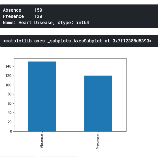
Our dataset has features that follow a categorical nature. However, while printing the data type of those columns, we observe that they are considered as integers and this might make our model to treat them as continuous values despite being discrete by nature.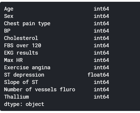
For this reason we will change explicitly their data type to categorical using astype() pandas method.
categorical_features = ["Sex", "Chest pain type", "FBS over 120", "EKG results", "Exercise angina", "Slope of ST", "Number of vessels fluro", "Thallium"]
df[categorical_features] = df[categorical_features].astype("category")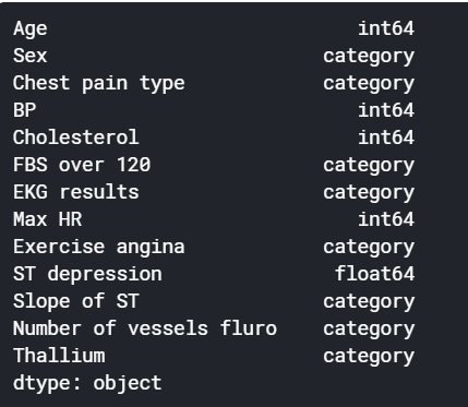
We will now scale our continuous features using MinMaxScaler, it is a type of normalization where the values will range between 0 and 1 and the equation is defined by X_Norm = (X - X_Min) / (X_Max - X_Min).
continuous_features = set(df.columns) - set(categorical_features)
scaler = MinMaxScaler()
df_norm = df.copy()
df_norm[list(continuous_features)] = scaler.fit_transform(df[list(continuous_features)])
Feature Selection Using Chi-Square
A chi-square test is used in statistics to test the independence of two events. Given the data of two variables, we can get observed count O and expected count E. Chi-Square measures how expected count E and observed count O deviates each other.
In feature selection, and since chi2 tests the degree of independence between two variables, we will use it between every feature and the label and we will keep only the k number of features with the highest chi2 value, because we want to keep only the features that are the most dependent of our label. We will important both SelectKBest and chi2 from sklearn.feature_selection module. SelectKBest requires two hyperparameter which are:
k: the number of features we want to select.score_func: the function on which the selection process is based upon.
X_new = SelectKBest(k=5, score_func=chi2).fit_transform(df_norm, label)Feature Selection Using Recursive Feature Elimination (RFE)
From sklearn Documentation: The goal of recursive feature elimination (RFE) is to select features by recursively considering smaller and smaller sets of features. We will be using sklearn.feature_selection module to import RFE class as well. RFE requires two hyperparameters:
n_features_to_select: the number of features we want to select.estimator: Which type of machine learning model will be used for the prediction in every iteration while recursively searching for the appropriate set of features.
rfe = RFE(estimator=RandomForestClassifier(), n_features_to_select=5)
X_new = rfe.fit_transform(df_norm, label)
X_new
Feature Selection Using Random Forest
Tree-based machine learning algorithms like DecisionTreeClassifier or their ensemble learning equivalent RandomForestClassifier uses a set of trees which contains nodes resulting from splitting. The main aim of those splits is to decrease impurity as much as possible by using impurity measures like entropy and gini index. Those tree-based models can calculate how much important a feature is by calculating the amount of impurity decrease this feature will lead to.
clf = RandomForestClassifier()
clf.fit(df_norm, label)
# create a figure to plot a bar, where x axis is features, and Y indicating the importance of each feature
plt.figure(figsize=(12,12))
plt.bar(df_norm.columns, clf.feature_importances_)
plt.xticks(rotation=45)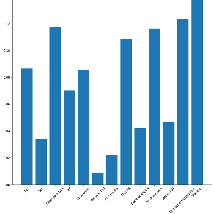
The above histogram shows the importance of each feature. In our case, Thallium and the number of vessels fluro are the most important features, but most of them have importance, and since that's the case, it's pretty much worth feeding these features to our machine learning model.
Now that you have selected the best features, you can easily use any sklearn classifier model and feed X_new array and see if it impacts the accuracy of the full features model.
Conclusion
Using such techniques for feature selection varies from one problem to another and also from a feature to another depending on their type being categorical or continuous.
In addition, the number of features to select can be answered by following an iterative approach until the k (in SelectKBest) converges, and the machine learning performance does not increase too much.
In this article, we have learned how to:
- Use chi2 to select the features that are highly dependent on the label.
- Use RFE to recursively find the optimal set of features given an estimator.
- Use tree-based machine learning methods like Random Forest to display the features that help to reduce as much as possible the impurity while splitting the nodes.
Related: How to Apply HOG Feature Extraction in Python.
Happy Learning ♥
Let our Code Converter simplify your multi-language projects. It's like having a coding translator at your fingertips. Don't miss out!
View Full Code Assist My Coding



Got a coding query or need some guidance before you comment? Check out this Python Code Assistant for expert advice and handy tips. It's like having a coding tutor right in your fingertips!