Before we get started, have you tried our new Python Code Assistant? It's like having an expert coder at your fingertips. Check it out!
Introduction
Financial institutions have many clients close their accounts or migrate to other institutions. As a result, this has made a significant hole in sales and may significantly impact yearly revenues for the current fiscal year, leading stocks to plummet and market value to fall by a decent percentage. A team of business, product, engineering, and data science professionals has been assembled to halt this decline.
The objective of this tutorial is that we want to build a model to predict, with reasonable accuracy, the customers who are going to churn soon.
A customer having closed all their active accounts with the bank is said to have churned. Churn can be defined in other ways as well, based on the context of the problem. A customer not transacting for six months or one year can also be defined as churned based on the business requirements.
Table of content:
- Introduction
- The Dataset
- Questioning the Data
- Exploratory Data Analysis
- Data Preprocessing
- Bivariate Analysis
- Feature Scaling and Normalization
- Feature Selection using RFE
- Baseline Model 1: Logistic Regression
- Baseline Model 2: Support Vector Machines
- Plotting Decision Boundaries of Linear Models
- Baseline Model 3 (Non-linear): Decision Tree Classifier
- Data Preparation Automatization and Model Run through Pipelines
- Saving the Optimal Model
- Getting the Churning Users on the Test Set
- Conclusion
The Dataset
In the customer churn modeling dataset, we have 10000 rows (each representing a unique customer) with 15 columns: 14 features with one target feature (Exited). The data is composed of both numerical and categorical features:
The target column:
Exited— Whether the customer churned or not.
Numeric Features:
CustomerId: A unique ID of the customer.CreditScore: The credit score of the customer,Age: The age of the customer,Tenure: The number of months the client has been with the firm.Balance: Balance remaining in the customer account,NumOfProducts: The number of products sold by the customer.EstimatedSalary: The estimated salary of the customer.
Categorical Features:
Surname: The surname of the customer.Geography: The country of the customer.Gender: M/FHasCrCard: Whether the customer has a credit card or not.IsActiveMember: Whether the customer is active or not.
If you don't have a Kaggle account, the dataset can be downloaded here or here.
Questioning the Data
Here, the objective is to understand the data further and distill the problem statement and the stated goal. In the process, if more data/context can be obtained, that adds to the result of the model performance:
- No date/time column. A lot of useful features can be built using date/time columns.
- When was the data snapshot taken? There are certain customer features like
Balance,Tenure,NumOfProducts,EstimatedSalary, which will have different values across time. - Are all these features about the same single date or spread across multiple dates?
- How frequently are customer features updated?
- Will it be possible to have the values of these features over some time as opposed to a single snapshot date?
- Some customers who have exited still have a balance in their account or a non-zero
NumOfProducts. Does this mean they had churned only from a specific product and not the entire bank, or are these snapshots just before they churned? - Some features like number and kind of transactions can help us estimate the degree of activity of the customer, instead of trusting the binary variable
IsActiveMember. - Customer transaction patterns can also help us ascertain whether the customer has churned or not. For example, a customer might transact daily/weekly vs. a customer who transacts annually.
We don't have answers to all of these questions, and we will only use what we have.
Once the dataset is downloaded, put it in the current working directory.
Let's install the dependencies of this tutorial:
$ pip install ipython==7.22.0 joblib==1.0.1 lightgbm==3.3.1 matplotlib numpy pandas scikit_learn==0.24.1 seaborn xgboost==1.5.1Let's import the libraries:
import pandas as pd
import numpy as np
import matplotlib.pyplot as plt
import seaborn as sns
from sklearn.preprocessing import LabelEncoder, OneHotEncoder, StandardScaler
from sklearn.feature_selection import RFE
from sklearn.linear_model import LogisticRegression
from sklearn.svm import SVC
from sklearn.decomposition import PCA
from sklearn.tree import DecisionTreeClassifier, export_graphviz
from sklearn.pipeline import Pipeline
from sklearn.model_selection import train_test_split
from lightgbm import LGBMClassifier
from sklearn.metrics import roc_auc_score, recall_score, confusion_matrix, classification_report
import subprocess
import joblib
# Get multiple outputs in the same cell
from IPython.core.interactiveshell import InteractiveShell
InteractiveShell.ast_node_interactivity = "all"
# Ignore all warnings
import warnings
warnings.filterwarnings('ignore')
warnings.filterwarnings(action='ignore', category=DeprecationWarning)
pd.set_option('display.max_columns', None)
pd.set_option('display.max_rows', None)
Reading the dataset:
# Reading the dataset
dc = pd.read_csv("Churn_Modelling.csv")
dc.head(5)
╔═══╤═══════════╤════════════╤══════════╤═════════════╤═══════════╤════════╤═════╤════════╤═══════════╤═══════════════╤═══════════╤════════════════╤═════════════════╤════════╗
║ │ RowNumber │ CustomerId │ Surname │ CreditScore │ Geography │ Gender │ Age │ Tenure │ Balance │ NumOfProducts │ HasCrCard │ IsActiveMember │ EstimatedSalary │ Exited ║
╠═══╪═══════════╪════════════╪══════════╪═════════════╪═══════════╪════════╪═════╪════════╪═══════════╪═══════════════╪═══════════╪════════════════╪═════════════════╪════════╣
║ 0 │ 1 │ 15634602 │ Hargrave │ 619 │ France │ Female │ 42 │ 2 │ 0.00 │ 1 │ 1 │ 1 │ 101348.88 │ 1 ║
╟───┼───────────┼────────────┼──────────┼─────────────┼───────────┼────────┼─────┼────────┼───────────┼───────────────┼───────────┼────────────────┼─────────────────┼────────╢
║ 1 │ 2 │ 15647311 │ Hill │ 608 │ Spain │ Female │ 41 │ 1 │ 83807.86 │ 1 │ 0 │ 1 │ 112542.58 │ 0 ║
╟───┼───────────┼────────────┼──────────┼─────────────┼───────────┼────────┼─────┼────────┼───────────┼───────────────┼───────────┼────────────────┼─────────────────┼────────╢
║ 2 │ 3 │ 15619304 │ Onio │ 502 │ France │ Female │ 42 │ 8 │ 159660.80 │ 3 │ 1 │ 0 │ 113931.57 │ 1 ║
╟───┼───────────┼────────────┼──────────┼─────────────┼───────────┼────────┼─────┼────────┼───────────┼───────────────┼───────────┼────────────────┼─────────────────┼────────╢
║ 3 │ 4 │ 15701354 │ Boni │ 699 │ France │ Female │ 39 │ 1 │ 0.00 │ 2 │ 0 │ 0 │ 93826.63 │ 0 ║
╟───┼───────────┼────────────┼──────────┼─────────────┼───────────┼────────┼─────┼────────┼───────────┼───────────────┼───────────┼────────────────┼─────────────────┼────────╢
║ 4 │ 5 │ 15737888 │ Mitchell │ 850 │ Spain │ Female │ 43 │ 2 │ 125510.82 │ 1 │ 1 │ 1 │ 79084.10 │ 0 ║
╚═══╧═══════════╧════════════╧══════════╧═════════════╧═══════════╧════════╧═════╧════════╧═══════════╧═══════════════╧═══════════╧════════════════╧═════════════════╧════════╝Related: Recommender Systems using Association Rules Mining in Python.
Exploratory Data Analysis
Let's see the dimension of the dataset:
# Dimension of the dataset
dc.shape
(10000, 14)Let's see some statistics of the data. The first line describes all numerical columns, where the second describes categorical columns:
dc.describe(exclude= ['O']) # Describe all numerical columns
dc.describe(include = ['O']) # Describe all categorical columns
╔═══════╤═════════════╤══════════════╤══════════════╤══════════════╤══════════════╤═══════════════╤═══════════════╤═════════════╤════════════════╤═════════════════╤══════════════╗
║ │ RowNumber │ CustomerId │ CreditScore │ Age │ Tenure │ Balance │ NumOfProducts │ HasCrCard │ IsActiveMember │ EstimatedSalary │ Exited ║
╠═══════╪═════════════╪══════════════╪══════════════╪══════════════╪══════════════╪═══════════════╪═══════════════╪═════════════╪════════════════╪═════════════════╪══════════════╣
║ count │ 10000.00000 │ 1.000000e+04 │ 10000.000000 │ 10000.000000 │ 10000.000000 │ 10000.000000 │ 10000.000000 │ 10000.00000 │ 10000.000000 │ 10000.000000 │ 10000.000000 ║
╟───────┼─────────────┼──────────────┼──────────────┼──────────────┼──────────────┼───────────────┼───────────────┼─────────────┼────────────────┼─────────────────┼──────────────╢
║ mean │ 5000.50000 │ 1.569094e+07 │ 650.528800 │ 38.921800 │ 5.012800 │ 76485.889288 │ 1.530200 │ 0.70550 │ 0.515100 │ 100090.239881 │ 0.203700 ║
╟───────┼─────────────┼──────────────┼──────────────┼──────────────┼──────────────┼───────────────┼───────────────┼─────────────┼────────────────┼─────────────────┼──────────────╢
║ std │ 2886.89568 │ 7.193619e+04 │ 96.653299 │ 10.487806 │ 2.892174 │ 62397.405202 │ 0.581654 │ 0.45584 │ 0.499797 │ 57510.492818 │ 0.402769 ║
╟───────┼─────────────┼──────────────┼──────────────┼──────────────┼──────────────┼───────────────┼───────────────┼─────────────┼────────────────┼─────────────────┼──────────────╢
║ min │ 1.00000 │ 1.556570e+07 │ 350.000000 │ 18.000000 │ 0.000000 │ 0.000000 │ 1.000000 │ 0.00000 │ 0.000000 │ 11.580000 │ 0.000000 ║
╟───────┼─────────────┼──────────────┼──────────────┼──────────────┼──────────────┼───────────────┼───────────────┼─────────────┼────────────────┼─────────────────┼──────────────╢
║ 25% │ 2500.75000 │ 1.562853e+07 │ 584.000000 │ 32.000000 │ 3.000000 │ 0.000000 │ 1.000000 │ 0.00000 │ 0.000000 │ 51002.110000 │ 0.000000 ║
╟───────┼─────────────┼──────────────┼──────────────┼──────────────┼──────────────┼───────────────┼───────────────┼─────────────┼────────────────┼─────────────────┼──────────────╢
║ 50% │ 5000.50000 │ 1.569074e+07 │ 652.000000 │ 37.000000 │ 5.000000 │ 97198.540000 │ 1.000000 │ 1.00000 │ 1.000000 │ 100193.915000 │ 0.000000 ║
╟───────┼─────────────┼──────────────┼──────────────┼──────────────┼──────────────┼───────────────┼───────────────┼─────────────┼────────────────┼─────────────────┼──────────────╢
║ 75% │ 7500.25000 │ 1.575323e+07 │ 718.000000 │ 44.000000 │ 7.000000 │ 127644.240000 │ 2.000000 │ 1.00000 │ 1.000000 │ 149388.247500 │ 0.000000 ║
╟───────┼─────────────┼──────────────┼──────────────┼──────────────┼──────────────┼───────────────┼───────────────┼─────────────┼────────────────┼─────────────────┼──────────────╢
║ max │ 10000.00000 │ 1.581569e+07 │ 850.000000 │ 92.000000 │ 10.000000 │ 250898.090000 │ 4.000000 │ 1.00000 │ 1.000000 │ 199992.480000 │ 1.000000 ║
╚═══════╧═════════════╧══════════════╧══════════════╧══════════════╧══════════════╧═══════════════╧═══════════════╧═════════════╧════════════════╧═════════════════╧══════════════╝
╔════════╤═════════╤═══════════╤════════╗
║ │ Surname │ Geography │ Gender ║
╠════════╪═════════╪═══════════╪════════╣
║ count │ 10000 │ 10000 │ 10000 ║
╟────────┼─────────┼───────────┼────────╢
║ unique │ 2932 │ 3 │ 2 ║
╟────────┼─────────┼───────────┼────────╢
║ top │ Smith │ France │ Male ║
╟────────┼─────────┼───────────┼────────╢
║ freq │ 32 │ 5014 │ 5457 ║
╚════════╧═════════╧═══════════╧════════╝Checking the number of unique customers:
# Checking number of unique customers in the dataset
dc.shape[0], dc.CustomerId.nunique()
(10000, 10000)This means each row corresponds to a customer.
Let's see the churn distribution:
# churn value Distribution
dc["Exited"].value_counts()
0 7963
1 2037
Name: Exited, dtype: int64The data set is imbalanced from the above result, with a significant chunk of existing customers relative to their churned peers.
Below, we group by Surname to see the average churn value:
dc.groupby(['Surname']).agg({'RowNumber':'count', 'Exited':'mean'}
                                  ).reset_index().sort_values(by='RowNumber', ascending=False).head()
╔══════╤═════════╤═══════════╤══════════╗
║ │ Surname │ RowNumber │ Exited ║
╠══════╪═════════╪═══════════╪══════════╣
║ 2473 │ Smith │ 32 │ 0.281250 ║
╟──────┼─────────┼───────────┼──────────╢
║ 1689 │ Martin │ 29 │ 0.310345 ║
╟──────┼─────────┼───────────┼──────────╢
║ 2389 │ Scott │ 29 │ 0.103448 ║
╟──────┼─────────┼───────────┼──────────╢
║ 2751 │ Walker │ 28 │ 0.142857 ║
╟──────┼─────────┼───────────┼──────────╢
║ 336 │ Brown │ 26 │ 0.192308 ║
╚══════╧═════════╧═══════════╧══════════╝Or grouping by Geography:
dc.groupby(['Geography']).agg({'RowNumber':'count', 'Exited':'mean'}
                                  ).reset_index().sort_values(by='RowNumber', ascending=False)
╔═══╤═══════════╤═══════════╤══════════╗
║ │ Geography │ RowNumber │ Exited ║
╠═══╪═══════════╪═══════════╪══════════╣
║ 0 │ France │ 5014 │ 0.161548 ║
╟───┼───────────┼───────────┼──────────╢
║ 1 │ Germany │ 2509 │ 0.324432 ║
╟───┼───────────┼───────────┼──────────╢
║ 2 │ Spain │ 2477 │ 0.166734 ║
╚═══╧═══════════╧═══════════╧══════════╝From what we see above, customers from Germany have a higher exiting rate than average.
Univariate Plots of Numerical Variables
Plotting CreditScore as a boxplot:
sns.set(style="whitegrid")
sns.boxplot(y=dc['CreditScore'])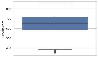
Age:
sns.boxplot(y=dc['Age'])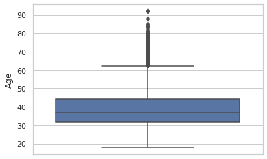
Tenure violin plot:
sns.violinplot(y = dc.Tenure)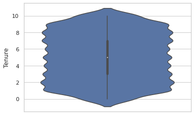
Balance:
sns.violinplot(y = dc['Balance'])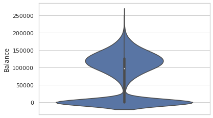
Plotting a distribution plot of NumOfProducts:
sns.set(style = 'ticks')
sns.distplot(dc.NumOfProducts, hist=True, kde=False)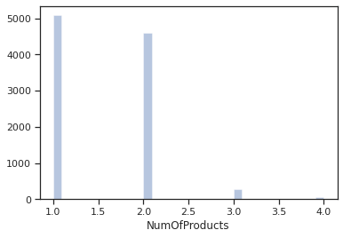
Most of the customers have 1 or 2 products.
Kernel density estimation plot for EstimatedSalary:
# When dealing with numerical characteristics, one of the most useful statistics to examine is the data distribution.
# we can use Kernel-Density-Estimation plot for that purpose.
sns.kdeplot(dc.EstimatedSalary)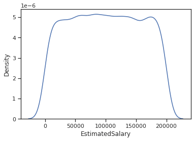
Data Preprocessing
So, in summary, here's what we're going to do:
- We will discard the
RowNumbercolumn. - We will discard
CustomerIDas well since it doesn't convey any extra info. Each row pertains to a unique customer. - Features can be segregated into non-essential, numerical, categorical, and target variables based on the above.
In general, CustomerID is a handy feature based on which we can calculate many user-centric features. Here, the dataset is not sufficient to calculate any extra customer features.
Let's define the types of columns we have:
# Separating out different columns into various categories as defined above
target_var = ['Exited']
cols_to_remove = ['RowNumber', 'CustomerId']
# numerical columns
num_feats = ['CreditScore', 'Age', 'Tenure', 'Balance', 'NumOfProducts', 'EstimatedSalary']
# categorical columns
cat_feats = ['Surname', 'Geography', 'Gender', 'HasCrCard', 'IsActiveMember']
Among these, Tenure and NumOfProducts are ordinal variables. HasCrCard and IsActiveMember are binary categorical variables.
Separating target variable and removing the non-essential columns:
y = dc[target_var].values
dc.drop(cols_to_remove, axis=1, inplace=True)
Splitting our Dataset
Since this is the only data available, we keep aside a test set to evaluate our model at the very end to estimate our chosen model's performance on unseen data. A validation set is also created, which we'll use in our baseline models to evaluate and tune our models:
# Keeping aside a test/holdout set
dc_train_val, dc_test, y_train_val, y_test = train_test_split(dc, y.ravel(), test_size = 0.1, random_state = 42)

# Splitting into train and validation set
dc_train, dc_val, y_train, y_val = train_test_split(dc_train_val, y_train_val, test_size = 0.12, random_state = 42)
dc_train.shape, dc_val.shape, dc_test.shape, y_train.shape, y_val.shape, y_test.shape
np.mean(y_train), np.mean(y_val), np.mean(y_test)
((7920, 12), (1080, 12), (1000, 12), (7920,), (1080,), (1000,))(0.20303030303030303, 0.22037037037037038, 0.191)Categorical Variable Encoding
We will use:
- Label Encoding: transforms non-numerical labels into numerical ones. It can be used for binary categorical and ordinal variables.
- One-Hot encoding: encodes categorical features as a one-hot numeric array. It can be used for non-ordinal categorical variables with low to mid cardinality (< 5-10 levels)
- Target encoding: the technique of substituting a categorical value with the mean of the target variable is known as target encoding. The target encoder model automatically removes any non-categorical columns. It can be used for Categorical variables with > 10 levels
HasCrCardandIsActiveMemberare already label encoded.- For
Gender, a simple label encoding should be acceptable. - For
Geography, since there are three levels, one-hot encoding should do the trick. - For
Surname, we'll try target/frequency encoding.
Label Encoding for Binary Variables
In this section, we will perform label encoding on the Gender column.
We only fit on the training set as that's the only data we'll assume we have. We'll treat validation and test sets as unseen data. Hence, they can't be used for fitting the encoders:
# label encoding With  the sklearn method
le = LabelEncoder()
# Label encoding of Gender variable
dc_train['Gender'] = le.fit_transform(dc_train['Gender'])
le_gender_mapping = dict(zip(le.classes_, le.transform(le.classes_)))
le_gender_mapping
{'Female': 0, 'Male': 1}For testing and validation sets:
# Encoding Gender feature for validation and test set
dc_val['Gender'] = dc_val.Gender.map(le_gender_mapping)
dc_test['Gender'] = dc_test.Gender.map(le_gender_mapping)

# Filling missing/NaN values created due to new categorical levels
dc_val['Gender'].fillna(-1, inplace=True)
dc_test['Gender'].fillna(-1, inplace=True)
Checking the values on all sets:
dc_train.Gender.unique(), dc_val.Gender.unique(), dc_test.Gender.unique()(array([1, 0]), array([1, 0]), array([1, 0]))One-hot Encoding Categorical Variables
Let's one-hot encode the Geography column:
# With the sklearn method(LabelEncoder())
le_ohe = LabelEncoder()
ohe = OneHotEncoder(handle_unknown = 'ignore', sparse=False)
enc_train = le_ohe.fit_transform(dc_train.Geography).reshape(dc_train.shape[0],1)
ohe_train = ohe.fit_transform(enc_train)
ohe_train
array([[0., 1., 0.],
[1., 0., 0.],
[1., 0., 0.],
...,
[1., 0., 0.],
[0., 1., 0.],
[0., 1., 0.]])# mapping between classes
le_ohe_geography_mapping = dict(zip(le_ohe.classes_, le_ohe.transform(le_ohe.classes_)))
le_ohe_geography_mapping{'France': 0, 'Germany': 1, 'Spain': 2}Now that we have the mapping dictionary, let's do the same for testing and validation sets:
# Encoding Geography feature for validation and test set
enc_val = dc_val.Geography.map(le_ohe_geography_mapping).ravel().reshape(-1,1)
enc_test = dc_test.Geography.map(le_ohe_geography_mapping).ravel().reshape(-1,1)

# Filling missing/NaN values created due to new categorical levels
enc_val[np.isnan(enc_val)] = 9999
enc_test[np.isnan(enc_test)] = 9999
ohe_val = ohe.transform(enc_val)
ohe_test = ohe.transform(enc_test)In case there is a country that isn't present in the training set, the resulting vector will simply be [0, 0, 0]:
# Show what happens when a new value is inputted into the OHE
ohe.transform(np.array([[9999]]))
array([[0., 0., 0.]])Adding the one-hot encoded columns to the data frame and removing the original feature:
cols = ['country_' + str(x) for x in le_ohe_geography_mapping.keys()]
cols
['country_France', 'country_Germany', 'country_Spain']# Adding to the respective dataframes
dc_train = pd.concat([dc_train.reset_index(), pd.DataFrame(ohe_train, columns = cols)], axis = 1).drop(['index'], axis=1)
dc_val = pd.concat([dc_val.reset_index(), pd.DataFrame(ohe_val, columns = cols)], axis = 1).drop(['index'], axis=1)
dc_test = pd.concat([dc_test.reset_index(), pd.DataFrame(ohe_test, columns = cols)], axis = 1).drop(['index'], axis=1)
print("Training set")
dc_train.head()
print("\n\nValidation set")
dc_val.head()
print("\n\nTest set")
dc_test.head()Training set
╔═══╤═══════════════╤═════════════╤═══════════╤════════╤═════╤════════╤═══════════╤═══════════════╤═══════════╤════════════════╤═════════════════╤════════╤════════════════╤═════════════════╤═══════════════╗
║ │ Surname │ CreditScore │ Geography │ Gender │ Age │ Tenure │ Balance │ NumOfProducts │ HasCrCard │ IsActiveMember │ EstimatedSalary │ Exited │ country_France │ country_Germany │ country_Spain ║
╠═══╪═══════════════╪═════════════╪═══════════╪════════╪═════╪════════╪═══════════╪═══════════════╪═══════════╪════════════════╪═════════════════╪════════╪════════════════╪═════════════════╪═══════════════╣
║ 0 │ Yermakova │ 678 │ Germany │ 1 │ 36 │ 1 │ 117864.85 │ 2 │ 1 │ 0 │ 27619.06 │ 0 │ 0.0 │ 1.0 │ 0.0 ║
╟───┼───────────────┼─────────────┼───────────┼────────┼─────┼────────┼───────────┼───────────────┼───────────┼────────────────┼─────────────────┼────────┼────────────────┼─────────────────┼───────────────╢
║ 1 │ Warlow-Davies │ 613 │ France │ 0 │ 27 │ 5 │ 125167.74 │ 1 │ 1 │ 0 │ 199104.52 │ 0 │ 1.0 │ 0.0 │ 0.0 ║
╟───┼───────────────┼─────────────┼───────────┼────────┼─────┼────────┼───────────┼───────────────┼───────────┼────────────────┼─────────────────┼────────┼────────────────┼─────────────────┼───────────────╢
║ 2 │ Fu │ 628 │ France │ 1 │ 45 │ 9 │ 0.00 │ 2 │ 1 │ 1 │ 96862.56 │ 0 │ 1.0 │ 0.0 │ 0.0 ║
╟───┼───────────────┼─────────────┼───────────┼────────┼─────┼────────┼───────────┼───────────────┼───────────┼────────────────┼─────────────────┼────────┼────────────────┼─────────────────┼───────────────╢
║ 3 │ Shih │ 513 │ France │ 1 │ 30 │ 5 │ 0.00 │ 2 │ 1 │ 0 │ 162523.66 │ 0 │ 1.0 │ 0.0 │ 0.0 ║
╟───┼───────────────┼─────────────┼───────────┼────────┼─────┼────────┼───────────┼───────────────┼───────────┼────────────────┼─────────────────┼────────┼────────────────┼─────────────────┼───────────────╢
║ 4 │ Mahmood │ 639 │ France │ 1 │ 22 │ 4 │ 0.00 │ 2 │ 1 │ 0 │ 28188.96 │ 0 │ 1.0 │ 0.0 │ 0.0 ║
╚═══╧═══════════════╧═════════════╧═══════════╧════════╧═════╧════════╧═══════════╧═══════════════╧═══════════╧════════════════╧═════════════════╧════════╧════════════════╧═════════════════╧═══════════════╝
Validation set
╔═══╤═════════╤═════════════╤═══════════╤════════╤═════╤════════╤═══════════╤═══════════════╤═══════════╤════════════════╤═════════════════╤════════╤════════════════╤═════════════════╤═══════════════╗
║ │ Surname │ CreditScore │ Geography │ Gender │ Age │ Tenure │ Balance │ NumOfProducts │ HasCrCard │ IsActiveMember │ EstimatedSalary │ Exited │ country_France │ country_Germany │ country_Spain ║
╠═══╪═════════╪═════════════╪═══════════╪════════╪═════╪════════╪═══════════╪═══════════════╪═══════════╪════════════════╪═════════════════╪════════╪════════════════╪═════════════════╪═══════════════╣
║ 0 │ Sun │ 757 │ France │ 1 │ 36 │ 7 │ 144852.06 │ 1 │ 0 │ 0 │ 130861.95 │ 0 │ 1.0 │ 0.0 │ 0.0 ║
╟───┼─────────┼─────────────┼───────────┼────────┼─────┼────────┼───────────┼───────────────┼───────────┼────────────────┼─────────────────┼────────┼────────────────┼─────────────────┼───────────────╢
║ 1 │ Russo │ 552 │ France │ 1 │ 29 │ 10 │ 0.00 │ 2 │ 1 │ 0 │ 12186.83 │ 0 │ 1.0 │ 0.0 │ 0.0 ║
╟───┼─────────┼─────────────┼───────────┼────────┼─────┼────────┼───────────┼───────────────┼───────────┼────────────────┼─────────────────┼────────┼────────────────┼─────────────────┼───────────────╢
║ 2 │ Munro │ 619 │ France │ 0 │ 30 │ 7 │ 70729.17 │ 1 │ 1 │ 1 │ 160948.87 │ 0 │ 1.0 │ 0.0 │ 0.0 ║
╟───┼─────────┼─────────────┼───────────┼────────┼─────┼────────┼───────────┼───────────────┼───────────┼────────────────┼─────────────────┼────────┼────────────────┼─────────────────┼───────────────╢
║ 3 │ Perkins │ 633 │ France │ 1 │ 35 │ 10 │ 0.00 │ 2 │ 1 │ 0 │ 65675.47 │ 0 │ 1.0 │ 0.0 │ 0.0 ║
╟───┼─────────┼─────────────┼───────────┼────────┼─────┼────────┼───────────┼───────────────┼───────────┼────────────────┼─────────────────┼────────┼────────────────┼─────────────────┼───────────────╢
║ 4 │ Aliyeva │ 698 │ Spain │ 1 │ 38 │ 10 │ 95010.92 │ 1 │ 1 │ 1 │ 105227.86 │ 0 │ 0.0 │ 0.0 │ 1.0 ║
╚═══╧═════════╧═════════════╧═══════════╧════════╧═════╧════════╧═══════════╧═══════════════╧═══════════╧════════════════╧═════════════════╧════════╧════════════════╧═════════════════╧═══════════════╝
Test set
╔═══╤══════════╤═════════════╤═══════════╤════════╤═════╤════════╤═══════════╤═══════════════╤═══════════╤════════════════╤═════════════════╤════════╤════════════════╤═════════════════╤═══════════════╗
║ │ Surname │ CreditScore │ Geography │ Gender │ Age │ Tenure │ Balance │ NumOfProducts │ HasCrCard │ IsActiveMember │ EstimatedSalary │ Exited │ country_France │ country_Germany │ country_Spain ║
╠═══╪══════════╪═════════════╪═══════════╪════════╪═════╪════════╪═══════════╪═══════════════╪═══════════╪════════════════╪═════════════════╪════════╪════════════════╪═════════════════╪═══════════════╣
║ 0 │ Anderson │ 596 │ Germany │ 1 │ 32 │ 3 │ 96709.07 │ 2 │ 0 │ 0 │ 41788.37 │ 0 │ 0.0 │ 1.0 │ 0.0 ║
╟───┼──────────┼─────────────┼───────────┼────────┼─────┼────────┼───────────┼───────────────┼───────────┼────────────────┼─────────────────┼────────┼────────────────┼─────────────────┼───────────────╢
║ 1 │ Herring │ 623 │ France │ 1 │ 43 │ 1 │ 0.00 │ 2 │ 1 │ 1 │ 146379.30 │ 0 │ 1.0 │ 0.0 │ 0.0 ║
╟───┼──────────┼─────────────┼───────────┼────────┼─────┼────────┼───────────┼───────────────┼───────────┼────────────────┼─────────────────┼────────┼────────────────┼─────────────────┼───────────────╢
║ 2 │ Amechi │ 601 │ Spain │ 0 │ 44 │ 4 │ 0.00 │ 2 │ 1 │ 0 │ 58561.31 │ 0 │ 0.0 │ 0.0 │ 1.0 ║
╟───┼──────────┼─────────────┼───────────┼────────┼─────┼────────┼───────────┼───────────────┼───────────┼────────────────┼─────────────────┼────────┼────────────────┼─────────────────┼───────────────╢
║ 3 │ Liang │ 506 │ Germany │ 1 │ 59 │ 8 │ 119152.10 │ 2 │ 1 │ 1 │ 170679.74 │ 0 │ 0.0 │ 1.0 │ 0.0 ║
╟───┼──────────┼─────────────┼───────────┼────────┼─────┼────────┼───────────┼───────────────┼───────────┼────────────────┼─────────────────┼────────┼────────────────┼─────────────────┼───────────────╢
║ 4 │ Chuang │ 560 │ Spain │ 0 │ 27 │ 7 │ 124995.98 │ 1 │ 1 │ 1 │ 114669.79 │ 0 │ 0.0 │ 0.0 │ 1.0 ║
╚═══╧══════════╧═════════════╧═══════════╧════════╧═════╧════════╧═══════════╧═══════════════╧═══════════╧════════════════╧═════════════════╧════════╧════════════════╧═════════════════╧═══════════════╝
Dropping the original Geography column now:
dc_train.drop(['Geography'], axis=1, inplace=True)
dc_val.drop(['Geography'], axis=1, inplace=True)
dc_test.drop(['Geography'], axis=1, inplace=True)
Target Encoding
Target encoding is generally proper when dealing with categorical variables of high cardinality (high number of levels). Here, we'll encode the Surname column (which has 2932 different values!) with the mean of the target variable for that level:
means = dc_train.groupby(['Surname']).Exited.mean()
means.head()
means.tail()
Surname
Abazu 0.00
Abbie 0.00
Abbott 0.25
Abdullah 1.00
Abdulov 0.00
Name: Exited, dtype: float64Surname
Zubarev 0.0
Zubareva 0.0
Zuev 0.0
Zuyev 0.0
Zuyeva 0.0
Name: Exited, dtype: float64Let's get the global mean of Exited column:
global_mean = y_train.mean()
global_mean0.20303030303030303# Creating new encoded features for surname - Target (mean) encoding
dc_train['Surname_mean_churn'] = dc_train.Surname.map(means)
dc_train['Surname_mean_churn'].fillna(global_mean, inplace=True)But, the problem with target encoding is that it might cause data leakage, as we are considering feedback from the target variable while computing any summary statistic. A solution is to use a modified version: Leave-one-out Target encoding; for a particular data point or row, the mean of the target is calculated by considering all rows in the same categorical level except itself. It mitigates data leakage and overfitting to some extent.
The mean for a category is mc = Sc / nc ..... (1), where Sc is the sum of the target variable for category c.
What we need to find is the mean excluding a single sample. This can be expressed as: mi = (Sc - ti) / (nc - 1) ..... (2)
Using (1) and (2), we can get: mi = (ncmc - ti) / (nc - 1)
where:
nc = number of rows in category c
ti = Target value of the row whose encoding is being calculated
Calculating the frequency of each Surname:
freqs = dc_train.groupby(['Surname']).size()
freqs.head()
Surname
Abazu 2
Abbie 1
Abbott 4
Abdullah 1
Abdulov 1
dtype: int64Create frequency encoding - Number of instances of each category in the data:
dc_train['Surname_freq'] = dc_train.Surname.map(freqs)
dc_train['Surname_freq'].fillna(0, inplace=True)
Creating Leave-one-out target encoding for Surname:
dc_train['Surname_enc'] = ((dc_train.Surname_freq * dc_train.Surname_mean_churn) - dc_train.Exited)/(dc_train.Surname_freq - 1)
# Fill NaNs occuring due to category frequency being 1 or less
dc_train['Surname_enc'].fillna((((dc_train.shape[0] * global_mean) - dc_train.Exited) / (dc_train.shape[0] - 1)), inplace=True)
dc_train.head(5)
╔═══╤═══════════════╤═════════════╤════════╤═════╤════════╤═══════════╤═══════════════╤═══════════╤════════════════╤═════════════════╤════════╤════════════════╤═════════════════╤═══════════════╤════════════════════╤══════════════╤═════════════╗
║ │ Surname │ CreditScore │ Gender │ Age │ Tenure │ Balance │ NumOfProducts │ HasCrCard │ IsActiveMember │ EstimatedSalary │ Exited │ country_France │ country_Germany │ country_Spain │ Surname_mean_churn │ Surname_freq │ Surname_enc ║
╠═══╪═══════════════╪═════════════╪════════╪═════╪════════╪═══════════╪═══════════════╪═══════════╪════════════════╪═════════════════╪════════╪════════════════╪═════════════════╪═══════════════╪════════════════════╪══════════════╪═════════════╣
║ 0 │ Yermakova │ 678 │ 1 │ 36 │ 1 │ 117864.85 │ 2 │ 1 │ 0 │ 27619.06 │ 0 │ 0.0 │ 1.0 │ 0.0 │ 0.000000 │ 4 │ 0.000000 ║
╟───┼───────────────┼─────────────┼────────┼─────┼────────┼───────────┼───────────────┼───────────┼────────────────┼─────────────────┼────────┼────────────────┼─────────────────┼───────────────┼────────────────────┼──────────────┼─────────────╢
║ 1 │ Warlow-Davies │ 613 │ 0 │ 27 │ 5 │ 125167.74 │ 1 │ 1 │ 0 │ 199104.52 │ 0 │ 1.0 │ 0.0 │ 0.0 │ 0.000000 │ 2 │ 0.000000 ║
╟───┼───────────────┼─────────────┼────────┼─────┼────────┼───────────┼───────────────┼───────────┼────────────────┼─────────────────┼────────┼────────────────┼─────────────────┼───────────────┼────────────────────┼──────────────┼─────────────╢
║ 2 │ Fu │ 628 │ 1 │ 45 │ 9 │ 0.00 │ 2 │ 1 │ 1 │ 96862.56 │ 0 │ 1.0 │ 0.0 │ 0.0 │ 0.200000 │ 10 │ 0.222222 ║
╟───┼───────────────┼─────────────┼────────┼─────┼────────┼───────────┼───────────────┼───────────┼────────────────┼─────────────────┼────────┼────────────────┼─────────────────┼───────────────┼────────────────────┼──────────────┼─────────────╢
║ 3 │ Shih │ 513 │ 1 │ 30 │ 5 │ 0.00 │ 2 │ 1 │ 0 │ 162523.66 │ 0 │ 1.0 │ 0.0 │ 0.0 │ 0.285714 │ 21 │ 0.300000 ║
╟───┼───────────────┼─────────────┼────────┼─────┼────────┼───────────┼───────────────┼───────────┼────────────────┼─────────────────┼────────┼────────────────┼─────────────────┼───────────────┼────────────────────┼──────────────┼─────────────╢
║ 4 │ Mahmood │ 639 │ 1 │ 22 │ 4 │ 0.00 │ 2 │ 1 │ 0 │ 28188.96 │ 0 │ 1.0 │ 0.0 │ 0.0 │ 0.333333 │ 3 │ 0.500000 ║
╚═══╧═══════════════╧═════════════╧════════╧═════╧════════╧═══════════╧═══════════════╧═══════════╧════════════════╧═════════════════╧════════╧════════════════╧═════════════════╧═══════════════╧════════════════════╧══════════════╧═════════════╝On validation and testing set, we'll apply the regular target encoding mapping as obtained from the training set:
# Replacing by category means and new category levels by global mean
dc_val['Surname_enc'] = dc_val.Surname.map(means)
dc_val['Surname_enc'].fillna(global_mean, inplace=True)
dc_test['Surname_enc'] = dc_test.Surname.map(means)
dc_test['Surname_enc'].fillna(global_mean, inplace=True)
# Show that using LOO Target encoding decorrelates features
dc_train[['Surname_mean_churn', 'Surname_enc', 'Exited']].corr()
╔════════════════════╤════════════════════╤═════════════════════════╗
║ │ Surname_mean_churn │ Surname_enc │ Exited ║
╠════════════════════╪════════════════════╪═════════════╪═══════════╣
║ Surname_mean_churn │ 1.000000 │ 0.54823 │ 0.562677 ║
╟────────────────────┼────────────────────┼─────────────┼───────────╢
║ Surname_enc │ 0.548230 │ 1.00000 │ -0.026440 ║
╟────────────────────┼────────────────────┼─────────────┼───────────╢
║ Exited │ 0.562677 │ -0.02644 │ 1.000000 ║
╚════════════════════╧════════════════════╧═════════════╧═══════════╝As you can see, Surname_enc isn't highly correlated with Exited as Surname_mean_churn, so Leave-one-out is effective here.
Deleting the Surname and other redundant columns across the three datasets:
dc_train.drop(['Surname_mean_churn'], axis=1, inplace=True)
dc_train.drop(['Surname_freq'], axis=1, inplace=True)
dc_train.drop(['Surname'], axis=1, inplace=True)
dc_val.drop(['Surname'], axis=1, inplace=True)
dc_test.drop(['Surname'], axis=1, inplace=True)
dc_train.head()
╔═══╤═════════════╤════════╤═════╤════════╤═══════════╤═══════════════╤═══════════╤════════════════╤═════════════════╤════════╤════════════════╤═════════════════╤═══════════════╤═════════════╗
║ │ CreditScore │ Gender │ Age │ Tenure │ Balance │ NumOfProducts │ HasCrCard │ IsActiveMember │ EstimatedSalary │ Exited │ country_France │ country_Germany │ country_Spain │ Surname_enc ║
╠═══╪═════════════╪════════╪═════╪════════╪═══════════╪═══════════════╪═══════════╪════════════════╪═════════════════╪════════╪════════════════╪═════════════════╪═══════════════╪═════════════╣
║ 0 │ 678 │ 1 │ 36 │ 1 │ 117864.85 │ 2 │ 1 │ 0 │ 27619.06 │ 0 │ 0.0 │ 1.0 │ 0.0 │ 0.000000 ║
╟───┼─────────────┼────────┼─────┼────────┼───────────┼───────────────┼───────────┼────────────────┼─────────────────┼────────┼────────────────┼─────────────────┼───────────────┼─────────────╢
║ 1 │ 613 │ 0 │ 27 │ 5 │ 125167.74 │ 1 │ 1 │ 0 │ 199104.52 │ 0 │ 1.0 │ 0.0 │ 0.0 │ 0.000000 ║
╟───┼─────────────┼────────┼─────┼────────┼───────────┼───────────────┼───────────┼────────────────┼─────────────────┼────────┼────────────────┼─────────────────┼───────────────┼─────────────╢
║ 2 │ 628 │ 1 │ 45 │ 9 │ 0.00 │ 2 │ 1 │ 1 │ 96862.56 │ 0 │ 1.0 │ 0.0 │ 0.0 │ 0.222222 ║
╟───┼─────────────┼────────┼─────┼────────┼───────────┼───────────────┼───────────┼────────────────┼─────────────────┼────────┼────────────────┼─────────────────┼───────────────┼─────────────╢
║ 3 │ 513 │ 1 │ 30 │ 5 │ 0.00 │ 2 │ 1 │ 0 │ 162523.66 │ 0 │ 1.0 │ 0.0 │ 0.0 │ 0.300000 ║
╟───┼─────────────┼────────┼─────┼────────┼───────────┼───────────────┼───────────┼────────────────┼─────────────────┼────────┼────────────────┼─────────────────┼───────────────┼─────────────╢
║ 4 │ 639 │ 1 │ 22 │ 4 │ 0.00 │ 2 │ 1 │ 0 │ 28188.96 │ 0 │ 1.0 │ 0.0 │ 0.0 │ 0.500000 ║
╚═══╧═════════════╧════════╧═════╧════════╧═══════════╧═══════════════╧═══════════╧════════════════╧═════════════════╧════════╧════════════════╧═════════════════╧═══════════════╧═════════════╝To summarize this section:
- Use label encoding and one-hot encoding on the training set and then save the mapping and apply it to the test set. For missing values, use 0, -1 etc.
- Target/Frequency encoding: Create a mapping between each level and a statistical measure (mean, median, sum, etc.) of the target from the training dataset. For the new categorical levels, impute the missing values suitably (can be 0, -1, or mean/mode/median).
- Leave-one-out or Cross-fold Target encoding avoids data leakage and helps generalize the model.
Bivariate Analysis
Let's check the linear correlation (rho) between individual features and the target variable:
corr = dc_train.corr()Drawing a heatmap:
sns.heatmap(corr, cmap = 'coolwarm')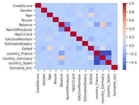
None of the features are highly correlated with the target variable. But some of them have slight linear associations with the target variable:
- Continuous features -
Age,Balance. - Categorical variables -
Gender,IsActiveMember,country_Germany,country_France.
Let's see individual features versus their distribution across target variable values, for Age column:
sns.boxplot(x="Exited", y="Age", data=dc_train, palette="Set3")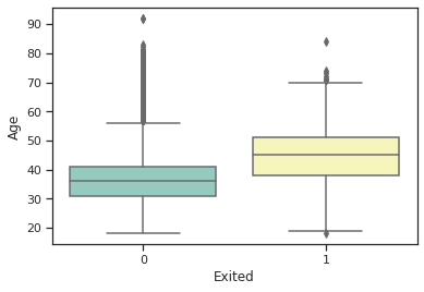
- There is an outside point at 90 for class 0 and 83 for class 1.
- The Median is around 35 for class 0 and 45 for class 1.
- The lower adjacent value is a bit less than 20 for both classes.
- The upper adjoining value is around 55 for class 0 and more than 70 for class 1.
A violin plot for the Balance:
sns.violinplot(x="Exited", y="Balance", data=dc_train, palette="Set3")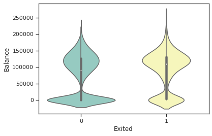
We can see a high probability of observation at 125000 (balance) and a peak at 0 (balance) for class 0
Checking association of categorical features with the target variable:
cat_vars_bv = ['Gender', 'IsActiveMember', 'country_Germany', 'country_France']

for col in cat_vars_bv:
    dc_train.groupby([col]).Exited.mean()
    print()
Gender
0 0.248191
1 0.165511
Name: Exited, dtype: float64
IsActiveMember
0 0.266285
1 0.143557
Name: Exited, dtype: float64
country_Germany
0.0 0.163091
1.0 0.324974
Name: Exited, dtype: float64
country_France
0.0 0.245877
1.0 0.160593
Name: Exited, dtype: float64From the above results, we can observe that the mean of the churned customer across Germany is higher than the others.
# Computed mean on churned or non chuned custmers group by number of product on training data
col = 'NumOfProducts'
dc_train.groupby([col]).Exited.mean()
# unique "NumOfProducts" on training data
dc_train[col].value_counts()
NumOfProducts
1 0.273428
2 0.076881
3 0.825112
4 1.000000
Name: Exited, dtype: float641 4023
2 3629
3 223
4 45
Name: NumOfProducts, dtype: int64All customers with four products have churned, and about 82.5% of customers with three products have churned.
Creating some new features based on simple interactions between the existing features:
eps = 1e-6

dc_train['bal_per_product'] = dc_train.Balance/(dc_train.NumOfProducts + eps)
dc_train['bal_by_est_salary'] = dc_train.Balance/(dc_train.EstimatedSalary + eps)
dc_train['tenure_age_ratio'] = dc_train.Tenure/(dc_train.Age + eps)
dc_train['age_surname_mean_churn'] = np.sqrt(dc_train.Age) * dc_train.Surname_enc
new_cols = ['bal_per_product', 'bal_by_est_salary', 'tenure_age_ratio', 'age_surname_mean_churn']
# Ensuring that the new column doesn't have any missing values
dc_train[new_cols].isnull().sum()bal_per_product 0
bal_by_est_salary 0
tenure_age_ratio 0
age_surname_mean_churn 0
dtype: int64# Linear association of new columns with target variables to judge importance
sns.heatmap(dc_train[new_cols + ['Exited']].corr(), annot=True)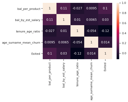
Out of the new features, ones with slight linear association/correlation are bal_per_product and tenure_age_ratio.
Let's create them on the validation and testing sets:
dc_val['bal_per_product'] = dc_val.Balance/(dc_val.NumOfProducts + eps)
dc_val['bal_by_est_salary'] = dc_val.Balance/(dc_val.EstimatedSalary + eps)
dc_val['tenure_age_ratio'] = dc_val.Tenure/(dc_val.Age + eps)
dc_val['age_surname_mean_churn'] = np.sqrt(dc_val.Age) * dc_val.Surname_enc
dc_test['bal_per_product'] = dc_test.Balance/(dc_test.NumOfProducts + eps)
dc_test['bal_by_est_salary'] = dc_test.Balance/(dc_test.EstimatedSalary + eps)
dc_test['tenure_age_ratio'] = dc_test.Tenure/(dc_test.Age + eps)
dc_test['age_surname_mean_churn'] = np.sqrt(dc_test.Age) * dc_test.Surname_enc
Feature Scaling and Normalization
Let's scale the continuous columns with the StandardScaler:
# initialize the standard scaler
sc = StandardScaler()
cont_vars = ['CreditScore', 'Age', 'Tenure', 'Balance', 'NumOfProducts', 'EstimatedSalary', 'Surname_enc', 'bal_per_product'
             , 'bal_by_est_salary', 'tenure_age_ratio', 'age_surname_mean_churn']
cat_vars = ['Gender', 'HasCrCard', 'IsActiveMember', 'country_France', 'country_Germany', 'country_Spain']
# Scaling only continuous columns
cols_to_scale = cont_vars
sc_X_train = sc.fit_transform(dc_train[cols_to_scale])
# Converting from array to dataframe and naming the respective features/columns
sc_X_train = pd.DataFrame(data=sc_X_train, columns=cols_to_scale)
sc_X_train.shape
sc_X_train.head()
(7920, 11)
╔═══╤═════════════╤═══════════╤═══════════╤═══════════╤═══════════════╤═════════════════╤═════════════╤═════════════════╤═══════════════════╤══════════════════╤════════════════════════╗
║ │ CreditScore │ Age │ Tenure │ Balance │ NumOfProducts │ EstimatedSalary │ Surname_enc │ bal_per_product │ bal_by_est_salary │ tenure_age_ratio │ age_surname_mean_churn ║
╠═══╪═════════════╪═══════════╪═══════════╪═══════════╪═══════════════╪═════════════════╪═════════════╪═════════════════╪═══════════════════╪══════════════════╪════════════════════════╣
║ 0 │ 0.284761 │ -0.274383 │ -1.389130 │ 0.670778 │ 0.804059 │ -1.254732 │ -1.079210 │ -0.062389 │ 0.095448 │ -1.232035 │ -1.062507 ║
╟───┼─────────────┼───────────┼───────────┼───────────┼───────────────┼─────────────────┼─────────────┼─────────────────┼───────────────────┼──────────────────┼────────────────────────╢
║ 1 │ -0.389351 │ -1.128482 │ -0.004763 │ 0.787860 │ -0.912423 │ 1.731950 │ -1.079210 │ 1.104840 │ -0.118834 │ 0.525547 │ -1.062507 ║
╟───┼─────────────┼───────────┼───────────┼───────────┼───────────────┼─────────────────┼─────────────┼─────────────────┼───────────────────┼──────────────────┼────────────────────────╢
║ 2 │ -0.233786 │ 0.579716 │ 1.379604 │ -1.218873 │ 0.804059 │ -0.048751 │ 0.094549 │ -1.100925 │ -0.155854 │ 0.690966 │ 0.193191 ║
╟───┼─────────────┼───────────┼───────────┼───────────┼───────────────┼─────────────────┼─────────────┼─────────────────┼───────────────────┼──────────────────┼────────────────────────╢
║ 3 │ -1.426446 │ -0.843782 │ -0.004763 │ -1.218873 │ 0.804059 │ 1.094838 │ 0.505364 │ -1.100925 │ -0.155854 │ 0.318773 │ 0.321611 ║
╟───┼─────────────┼───────────┼───────────┼───────────┼───────────────┼─────────────────┼─────────────┼─────────────────┼───────────────────┼──────────────────┼────────────────────────╢
║ 4 │ -0.119706 │ -1.602981 │ -0.350855 │ -1.218873 │ 0.804059 │ -1.244806 │ 1.561746 │ -1.100925 │ -0.155854 │ 0.487952 │ 0.912973 ║
╚═══╧═════════════╧═══════════╧═══════════╧═══════════╧═══════════════╧═════════════════╧═════════════╧═════════════════╧═══════════════════╧══════════════════╧════════════════════════╝# Scaling validation and test sets by transforming the mapping obtained through the training set
sc_X_val = sc.transform(dc_val[cols_to_scale])
sc_X_test = sc.transform(dc_test[cols_to_scale])
# Converting val and test arrays to dataframes for re-usability
sc_X_val = pd.DataFrame(data=sc_X_val, columns=cols_to_scale)
sc_X_test = pd.DataFrame(data=sc_X_test, columns=cols_to_scale)Feature scaling is essential for algorithms like Logistic Regression and SVM. It is not necessarily crucial for tree-based models such as decision trees.
Feature Selection using RFE
We can perform feature selection by eliminating features from the training dataset through Recursive Feature Elimination (RFE).
Features shortlisted through EDA/manual inspection and bivariate analysis: Age, Gender, Balance, NumOfProducts, IsActiveMember, the three Geography variables, bal_per_product, tenure_age_ratio.
Now, let's see whether feature selection and elimination through RFE give us the same list of features, other extra features, or a lesser number of features. To begin with, we'll feed all features to the RFE and LogReg model.
# Creating feature-set and target for RFE model
y = dc_train['Exited'].values
X = dc_train[cat_vars + cont_vars]
X.columns = cat_vars + cont_vars
X.columns
Index(['Gender', 'HasCrCard', 'IsActiveMember', 'country_France',
'country_Germany', 'country_Spain', 'CreditScore', 'Age', 'Tenure',
'Balance', 'NumOfProducts', 'EstimatedSalary', 'Surname_enc',
'bal_per_product', 'bal_by_est_salary', 'tenure_age_ratio',
'age_surname_mean_churn'],
dtype='object')We want to select ten features (you can change that if you wish to), so we set n_features_to_select as 10:
# for logistics regression
rfe = RFE(estimator=LogisticRegression(), n_features_to_select=10)
rfe = rfe.fit(X.values, y)
# mask of selected features
print(rfe.support_)
# The feature ranking, such that ranking_[i] corresponds to the ranking position of the i-th feature
print(rfe.ranking_)
We've printed the selected features as well as the ranking of the feature by importance:
[ True  True  True  True  True  True False  True False False  True False
  True False False  True False]
[1 1 1 1 1 1 4 1 3 6 1 8 1 7 5 1 2]
# Logistic regression (linear)
mask = rfe.support_.tolist()
selected_feats = [b for a,b in zip(mask, X.columns) if a]
selected_featsHere are the features that were chosen on logistic regression:
['Gender',
 'HasCrCard',
 'IsActiveMember',
 'country_France',
 'country_Germany',
 'country_Spain',
 'Age',
 'NumOfProducts',
 'Surname_enc',
 'tenure_age_ratio']
For the decision tree model:
rfe_dt = RFE(estimator=DecisionTreeClassifier(max_depth = 4, criterion = 'entropy'), n_features_to_select=10)
rfe_dt = rfe_dt.fit(X.values, y)
mask = rfe_dt.support_.tolist()
selected_feats_dt = [b for a,b in zip(mask, X.columns) if a]
selected_feats_dt['IsActiveMember',
'country_Germany',
'Age',
'Balance',
'NumOfProducts',
'EstimatedSalary',
'bal_per_product',
'bal_by_est_salary',
'tenure_age_ratio',
'age_surname_mean_churn']Baseline Model 1: Logistic Regression
We'll train the linear models on the features selected with RFE:
selected_cat_vars = [x for x in selected_feats if x in cat_vars]
selected_cont_vars = [x for x in selected_feats if x in cont_vars]
# Using categorical features and scaled numerical features
X_train = np.concatenate((dc_train[selected_cat_vars].values, sc_X_train[selected_cont_vars].values), axis=1)
X_val = np.concatenate((dc_val[selected_cat_vars].values, sc_X_val[selected_cont_vars].values), axis=1)
X_test = np.concatenate((dc_test[selected_cat_vars].values, sc_X_test[selected_cont_vars].values), axis=1)
# print the shapes
X_train.shape, X_val.shape, X_test.shape
((7920, 10), (1080, 10), (1000, 10))During the training phase, the weight differential will affect the classification of the classes. The overall goal is to penalize the minority class for misclassification by increasing class weight while decreasing weight for the majority class:
# Obtaining class weights based on the class samples imbalance ratio
_, num_samples = np.unique(y_train, return_counts=True)
weights = np.max(num_samples)/num_samples
# Define weight dictionnary
weights_dict = dict()
class_labels = [0,1]
# Weights associated with classes
for a,b in zip(class_labels,weights):
    weights_dict[a] = b

weights_dict
{0: 1.0, 1: 3.925373134328358}Let's retrain with class_weight:
# Defining model
lr = LogisticRegression(C=1.0, penalty='l2', class_weight=weights_dict, n_jobs=-1)
# train
lr.fit(X_train, y_train)
print(f'Confusion Matrix: \n{confusion_matrix(y_val, lr.predict(X_val))}')
print(f'Area Under Curve: {roc_auc_score(y_val, lr.predict(X_val))}')
print(f'Recall score: {recall_score(y_val,lr.predict(X_val))}')
print(f'Classification report: \n{classification_report(y_val,lr.predict(X_val))}')
Confusion Matrix:
[[590 252]
[ 71 167]]
Area Under Curve: 0.7011966306712709
Recall score: 0.7016806722689075
Classification report:
precision recall f1-score support
0 0.89 0.70 0.79 842
1 0.40 0.70 0.51 238
accuracy 0.70 1080
macro avg 0.65 0.70 0.65 1080
weighted avg 0.78 0.70 0.72 1080Baseline Model 2: Support Vector Machines
Let's train an SVC:
svm = SVC(C=1.0, kernel="linear", class_weight=weights_dict)
svm.fit(X_train, y_train)
# Validation metrics
print(f'Confusion Matrix: {confusion_matrix(y_val, lr.predict(X_val))}')
print(f'Area Under Curve: {roc_auc_score(y_val, lr.predict(X_val))}')
print(f'Recall score: {recall_score(y_val,lr.predict(X_val))}')
print(f'Classification report: \n{classification_report(y_val,lr.predict(X_val))}')Confusion Matrix: [[590 252]
[ 71 167]]
Area Under Curve: 0.7011966306712709
Recall score: 0.7016806722689075
Classification report:
precision recall f1-score support
0 0.89 0.70 0.79 842
1 0.40 0.70 0.51 238
accuracy 0.70 1080
macro avg 0.65 0.70 0.65 1080
weighted avg 0.78 0.70 0.72 1080Plotting Decision Boundaries of Linear Models
To plot the decision boundaries of classification models in a 2-D space, we first need to train our models in a 2D space. The best option is to use our existing data (with > 2 features) and apply dimensionality reduction techniques (like PCA) to it and then train our models on this data with a reduced number of features.
We will create an image in Meshgrid in which each pixel represents a grid cell in the 2D feature space. Over the 2D feature space, the image creates a grid. The classifier is used to classify the image's pixels, assigning a class label to each grid cell. The identified image is then utilized as the backdrop for a scatter plot with data points from each class.
pca = PCA(n_components=2)
# Transforming the dataset using PCA
X_pca = pca.fit_transform(X_train)
y = y_train
X_pca.shape, y.shape
((7920, 2), (7920,))# min and max values
xmin, xmax = X_pca[:, 0].min() - 2, X_pca[:, 0].max() + 2
ymin, ymax = X_pca[:, 1].min() - 2, X_pca[:, 1].max() + 2
# Creating a mesh region where the boundary will be plotted
xx, yy = np.meshgrid(np.arange(xmin, xmax, 0.2),
np.arange(ymin, ymax, 0.2))
# Fitting LR model on 2 features
lr.fit(X_pca, y)
# Fitting SVM model on 2 features
svm.fit(X_pca, y)
# Plotting decision boundary for LR
z1 = lr.predict(np.c_[xx.ravel(), yy.ravel()])
z1 = z1.reshape(xx.shape)
# Plotting decision boundary for SVM
z2 = svm.predict(np.c_[xx.ravel(), yy.ravel()])
z2 = z2.reshape(xx.shape)
# Displaying the result
plt.contourf(xx, yy, z1, alpha=0.4) # LR
plt.contour(xx, yy, z2, alpha=0.4, colors='blue') # SVM
sns.scatterplot(X_pca[:,0], X_pca[:,1], hue=y_train, s=50, alpha=0.8)
plt.title('Linear models - LogReg and SVM')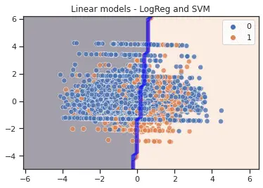
- Logistic regression estimator uses a linear separator for decision boundary.
- The Support Vector Machine finds a hyperplane with the maximum margin that divides the feature space into two classes.
- Decision Dense sampling with mesh grid may be used to illustrate decision boundary. However, the boundaries will seem erroneous if the grid resolution is insufficient. Mesh grid aims to generate a rectangular grid from an array of x values and an array of y values. We can find a detailed description of plotting a mesh grid here.
Baseline Model 3 (Non-linear): Decision Tree Classifier
Decision Trees are among the easiest algorithms to grasp, and their rationale is straightforward to explain:
# Features selected from the RFE process
selected_feats_dt
['IsActiveMember',
'country_Germany',
'Age',
'Balance',
'NumOfProducts',
'EstimatedSalary',
'bal_per_product',
'bal_by_est_salary',
'tenure_age_ratio',
'age_surname_mean_churn']# Re-defining X_train and X_val to consider original unscaled continuous features. y_train and y_val remain unaffected
X_train = dc_train[selected_feats_dt].values
X_val = dc_val[selected_feats_dt].values
# Decision tree classiier model
clf = DecisionTreeClassifier(criterion='entropy', class_weight=weights_dict, max_depth=4, max_features=None
, min_samples_split=25, min_samples_leaf=15)
# Fit the model
clf.fit(X_train, y_train)
# Checking the importance of different features of the model
pd.DataFrame({'features': selected_feats,
'importance': clf.feature_importances_
}).sort_values(by='importance', ascending=False)╔═══╤══════════════════╤════════════╗
║ │ features │ importance ║
╠═══╪══════════════════╪════════════╣
║ 2 │ IsActiveMember │ 0.476841 ║
╟───┼──────────────────┼────────────╢
║ 4 │ country_Germany │ 0.351863 ║
╟───┼──────────────────┼────────────╢
║ 0 │ Gender │ 0.096402 ║
╟───┼──────────────────┼────────────╢
║ 6 │ Age │ 0.032268 ║
╟───┼──────────────────┼────────────╢
║ 1 │ HasCrCard │ 0.028361 ║
╟───┼──────────────────┼────────────╢
║ 7 │ NumOfProducts │ 0.010400 ║
╟───┼──────────────────┼────────────╢
║ 5 │ country_Spain │ 0.003865 ║
╟───┼──────────────────┼────────────╢
║ 3 │ country_France │ 0.000000 ║
╟───┼──────────────────┼────────────╢
║ 8 │ Surname_enc │ 0.000000 ║
╟───┼──────────────────┼────────────╢
║ 9 │ tenure_age_ratio │ 0.000000 ║
╚═══╧══════════════════╧════════════╝IsActiveMember, country_Germany, Gender are the most important features for a decision tree.
Evaluating the model on training and validation dataset:
# Validation metrics
print(f'Confusion Matrix: {confusion_matrix(y_val, clf.predict(X_val))}')
print(f'Area Under Curve: {roc_auc_score(y_val, clf.predict(X_val))}')
print(f'Recall score: {recall_score(y_val,clf.predict(X_val))}')
print(f'Classification report: \n{classification_report(y_val,clf.predict(X_val))}')
Confusion Matrix: [[633 209]
[ 61 177]]
Area Under Curve: 0.7477394758378411
Recall score: 0.7436974789915967
Classification report:
precision recall f1-score support
0 0.91 0.75 0.82 842
1 0.46 0.74 0.57 238
accuracy 0.75 1080
macro avg 0.69 0.75 0.70 1080
weighted avg 0.81 0.75 0.77 1080We got better metrics here, 0.7 as a macro average of F1-score and 0.77 as a weighted average.
Let's perform decision tree rule engine visualization, which is a helpful tool to understand your model:
# Decision tree Classifier
clf = DecisionTreeClassifier(criterion='entropy', class_weight=weights_dict,
                            max_depth=3, max_features=None,
                            min_samples_split=25, min_samples_leaf=15)
# We fit the model
clf.fit(X_train, y_train)
# Export now as a dot file
dot_data = export_graphviz(clf, out_file='tree.dot',
                          feature_names=selected_feats_dt,
                          class_names=['Did not churn', 'Churned'],
                          rounded=True, proportion=False,
                          precision=2, filled=True)
# Convert to png using system command (requires Graphviz)
subprocess.run(['dot', '-Tpng','tree.dot', '-o', 'tree.png', '-Gdpi=600'])
# Display the rule-set of a single tree
from IPython.display import Image
Image(filename='tree.png')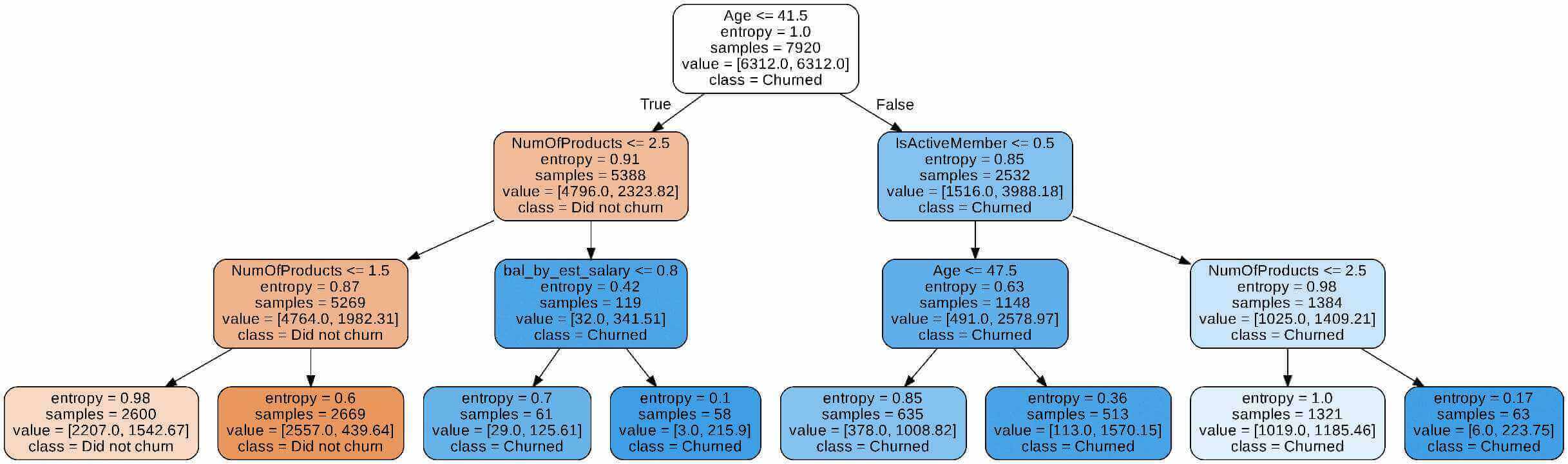
In the program above,
- We create and train a model.
- The
export_graphviz()function creates a GraphViz representation of the decision tree. - Using a system command, we can convert the dot to png with the
subprocess.run()method command. - We visualize the image by calling the function
Image(filename = 'tree.png'). - Entropy is a measure of the unpredictability of the information being processed. The greater the entropy, the more difficult it is to make inferences from the information.
- This decision tree reveals that the model is a series of logical questions and answers similar to what humans would develop when making predictions.
Data Preparation Automatization and Model Run through Pipelines
In this section, we will define three main classes:
- We create a sklearn transformer class, namely
CategoricalEncoderto perform label encoding, one-hot encoding, and target encoding. We draw our inspiration from this link. AddFeaturesclass that allows us to add newly engineered features using original categorical and numerical features of the DataFrame.CustomScalerthat can apply scaling on selected columns.
Since there is a lot of code, please get the utils.py file here and put it in the working directory.
After doing grid and randomized searches, we conclude that LGBMClassifier() outperforms all other models (you can get complete the code for searching in the original lengthy notebook).
from utils import *

# Preparing data and a few common model parameters
# Unscaled features will be used since it's a tree model

X_train = dc_train.drop(columns = ['Exited'], axis=1)
X_val = dc_val.drop(columns = ['Exited'], axis=1)

best_f1_lgb = LGBMClassifier(boosting_type='dart', class_weight={0: 1, 1: 3.0}, min_child_samples=20, n_jobs=-1, importance_type='gain', max_depth=6, num_leaves=63, colsample_bytree=0.6, learning_rate=0.1, n_estimators=201, reg_alpha=1, reg_lambda=1)
best_recall_lgb = LGBMClassifier(boosting_type='dart', num_leaves=31, max_depth=6, learning_rate=0.1, n_estimators=21, class_weight={0: 1, 1: 3.93}, min_child_samples=2, colsample_bytree=0.6, reg_alpha=0.3, reg_lambda=1.0, n_jobs=-1, importance_type='gain')
model = Pipeline(steps = [('categorical_encoding', CategoricalEncoder()),
                          ('add_new_features', AddFeatures()),
                          ('classifier', best_f1_lgb)
                         ])
# Fitting final model on train dataset
model.fit(X_train, y_train)
# Predict target probabilities
val_probs = model.predict_proba(X_val)[:,1]
# Predict target values on val data
val_preds = np.where(val_probs > 0.45, 1, 0) # The probability threshold can be tweaked
# Validation metrics
print(f'Confusion Matrix: {confusion_matrix(y_val,val_preds)}')
print(f'Area Under Curve: {roc_auc_score(y_val,val_preds)}')
print(f'Recall score: {recall_score(y_val,val_preds)}')
print(f'Classification report: \n{classification_report(y_val,val_preds)}')
Area Under Curve: 0.7587576598335297
Recall score: 0.6386554621848739
Classification report:
precision recall f1-score support
0 0.90 0.88 0.89 842
1 0.60 0.64 0.62 238
accuracy 0.83 1080
macro avg 0.75 0.76 0.75 1080
weighted avg 0.83 0.83 0.83 1080Saving the Optimal Model
Let's save the model using joblib:
# Save model object
joblib.dump(model, 'final_churn_model_f1_0_45.sav')
Getting the Churning Users on the Test Set
Here, we'll use dc_test as the unseen, future data:
# Load model object
model = joblib.load('final_churn_model_f1_0_45.sav')
X_test = dc_test.drop(columns=['Exited'], axis=1)
# Predict target probabilities
test_probs = model.predict_proba(X_test)[:,1]
# Predict target values on test data
test_preds = np.where(test_probs > 0.45, 1, 0) # Flexibility to tweak the probability threshold
#test_preds = model.predict(X_test)
# Test set metrics
roc_auc_score(y_test, test_preds)
recall_score(y_test, test_preds)
confusion_matrix(y_test, test_preds)
print(classification_report(y_test, test_preds))
0.76785702729114210.675392670157068array([[696, 113],
[ 62, 129]]) precision recall f1-score support
0 0.92 0.86 0.89 809
1 0.53 0.68 0.60 191
accuracy 0.82 1000
macro avg 0.73 0.77 0.74 1000
weighted avg 0.84 0.82 0.83 1000# Adding predictions and their probabilities in the original test dataframe
test = dc_test.copy()
test['predictions'] = test_preds
test['pred_probabilities'] = test_probs
test.sample(5)╔═════╤═════════════╤════════╤═════╤════════╤═══════════╤═══════════════╤═══════════╤════════════════╤═════════════════╤════════╤════════════════╤═════════════════╤═══════════════╤═════════════╤═════════════════╤═══════════════════╤══════════════════╤════════════════════════╤═════════════╤════════════════════╗
║ │ CreditScore │ Gender │ Age │ Tenure │ Balance │ NumOfProducts │ HasCrCard │ IsActiveMember │ EstimatedSalary │ Exited │ country_France │ country_Germany │ country_Spain │ Surname_enc │ bal_per_product │ bal_by_est_salary │ tenure_age_ratio │ age_surname_mean_churn │ predictions │ pred_probabilities ║
╠═════╪═════════════╪════════╪═════╪════════╪═══════════╪═══════════════╪═══════════╪════════════════╪═════════════════╪════════╪════════════════╪═════════════════╪═══════════════╪═════════════╪═════════════════╪═══════════════════╪══════════════════╪════════════════════════╪═════════════╪════════════════════╣
║ 612 │ 795 │ 0 │ 33 │ 9 │ 130862.43 │ 1 │ 1 │ 1 │ 114935.21 │ 0 │ 0.0 │ 1.0 │ 0.0 │ 0.000000 │ 130862.299138 │ 1.138576 │ 0.272727 │ 0.000000 │ 1 │ 0.504252 ║
╟─────┼─────────────┼────────┼─────┼────────┼───────────┼───────────────┼───────────┼────────────────┼─────────────────┼────────┼────────────────┼─────────────────┼───────────────┼─────────────┼─────────────────┼───────────────────┼──────────────────┼────────────────────────┼─────────────┼────────────────────╢
║ 241 │ 430 │ 1 │ 36 │ 1 │ 138992.48 │ 2 │ 0 │ 0 │ 122373.42 │ 0 │ 0.0 │ 1.0 │ 0.0 │ 0.222222 │ 69496.205252 │ 1.135806 │ 0.027778 │ 1.333333 │ 0 │ 0.161264 ║
╟─────┼─────────────┼────────┼─────┼────────┼───────────┼───────────────┼───────────┼────────────────┼─────────────────┼────────┼────────────────┼─────────────────┼───────────────┼─────────────┼─────────────────┼───────────────────┼──────────────────┼────────────────────────┼─────────────┼────────────────────╢
║ 999 │ 793 │ 1 │ 56 │ 8 │ 119496.25 │ 2 │ 1 │ 0 │ 29880.99 │ 0 │ 1.0 │ 0.0 │ 0.0 │ 0.285714 │ 59748.095126 │ 3.999073 │ 0.142857 │ 2.138090 │ 1 │ 0.828994 ║
╟─────┼─────────────┼────────┼─────┼────────┼───────────┼───────────────┼───────────┼────────────────┼─────────────────┼────────┼────────────────┼─────────────────┼───────────────┼─────────────┼─────────────────┼───────────────────┼──────────────────┼────────────────────────┼─────────────┼────────────────────╢
║ 177 │ 477 │ 0 │ 58 │ 8 │ 145984.92 │ 1 │ 1 │ 1 │ 24564.70 │ 0 │ 0.0 │ 1.0 │ 0.0 │ 0.203030 │ 145984.774015 │ 5.942874 │ 0.137931 │ 1.546233 │ 0 │ 0.246498 ║
╟─────┼─────────────┼────────┼─────┼────────┼───────────┼───────────────┼───────────┼────────────────┼─────────────────┼────────┼────────────────┼─────────────────┼───────────────┼─────────────┼─────────────────┼───────────────────┼──────────────────┼────────────────────────┼─────────────┼────────────────────╢
║ 495 │ 814 │ 0 │ 31 │ 4 │ 0.00 │ 2 │ 1 │ 1 │ 142029.17 │ 0 │ 1.0 │ 0.0 │ 0.0 │ 0.203030 │ 0.000000 │ 0.000000 │ 0.129032 │ 1.130425 │ 0 │ 0.012187 ║
╚═════╧═════════════╧════════╧═════╧════════╧═══════════╧═══════════════╧═══════════╧════════════════╧═════════════════╧════════╧════════════════╧═════════════════╧═══════════════╧═════════════╧═════════════════╧═══════════════════╧══════════════════╧════════════════════════╧═════════════╧════════════════════╝Listing customers who have a churn probability higher than 70% sorted by probability, these are the ones who can be targeted immediately:
high_churn_list = test[test.pred_probabilities > 0.7].sort_values(by=['pred_probabilities'], ascending=False
                                                                 ).reset_index().drop(columns=['index', 'Exited', 'predictions'], axis=1)
high_churn_list.shape
high_churn_list.head()
(103, 18)
╔═══╤═════════════╤════════╤═════╤════════╤═══════════╤═══════════════╤═══════════╤════════════════╤═════════════════╤════════════════╤═════════════════╤═══════════════╤═════════════╤═════════════════╤═══════════════════╤══════════════════╤════════════════════════╤════════════════════╗
║ │ CreditScore │ Gender │ Age │ Tenure │ Balance │ NumOfProducts │ HasCrCard │ IsActiveMember │ EstimatedSalary │ country_France │ country_Germany │ country_Spain │ Surname_enc │ bal_per_product │ bal_by_est_salary │ tenure_age_ratio │ age_surname_mean_churn │ pred_probabilities ║
╠═══╪═════════════╪════════╪═════╪════════╪═══════════╪═══════════════╪═══════════╪════════════════╪═════════════════╪════════════════╪═════════════════╪═══════════════╪═════════════╪═════════════════╪═══════════════════╪══════════════════╪════════════════════════╪════════════════════╣
║ 0 │ 546 │ 0 │ 58 │ 3 │ 106458.31 │ 4 │ 1 │ 0 │ 128881.87 │ 0.0 │ 1.0 │ 0.0 │ 0.000000 │ 26614.570846 │ 0.826015 │ 0.051724 │ 0.000000 │ 0.992935 ║
╟───┼─────────────┼────────┼─────┼────────┼───────────┼───────────────┼───────────┼────────────────┼─────────────────┼────────────────┼─────────────────┼───────────────┼─────────────┼─────────────────┼───────────────────┼──────────────────┼────────────────────────┼────────────────────╢
║ 1 │ 479 │ 1 │ 51 │ 1 │ 107714.74 │ 3 │ 1 │ 0 │ 86128.21 │ 0.0 │ 1.0 │ 0.0 │ 0.333333 │ 35904.901365 │ 1.250633 │ 0.019608 │ 2.380476 │ 0.979605 ║
╟───┼─────────────┼────────┼─────┼────────┼───────────┼───────────────┼───────────┼────────────────┼─────────────────┼────────────────┼─────────────────┼───────────────┼─────────────┼─────────────────┼───────────────────┼──────────────────┼────────────────────────┼────────────────────╢
║ 2 │ 745 │ 1 │ 45 │ 10 │ 117231.63 │ 3 │ 1 │ 1 │ 122381.02 │ 0.0 │ 1.0 │ 0.0 │ 0.250000 │ 39077.196974 │ 0.957923 │ 0.222222 │ 1.677051 │ 0.976361 ║
╟───┼─────────────┼────────┼─────┼────────┼───────────┼───────────────┼───────────┼────────────────┼─────────────────┼────────────────┼─────────────────┼───────────────┼─────────────┼─────────────────┼───────────────────┼──────────────────┼────────────────────────┼────────────────────╢
║ 3 │ 515 │ 1 │ 45 │ 7 │ 120961.50 │ 3 │ 1 │ 1 │ 39288.11 │ 0.0 │ 1.0 │ 0.0 │ 0.200000 │ 40320.486560 │ 3.078832 │ 0.155556 │ 1.341641 │ 0.970001 ║
╟───┼─────────────┼────────┼─────┼────────┼───────────┼───────────────┼───────────┼────────────────┼─────────────────┼────────────────┼─────────────────┼───────────────┼─────────────┼─────────────────┼───────────────────┼──────────────────┼────────────────────────┼────────────────────╢
║ 4 │ 481 │ 0 │ 57 │ 9 │ 0.00 │ 3 │ 1 │ 1 │ 169719.35 │ 1.0 │ 0.0 │ 0.0 │ 0.222222 │ 0.000000 │ 0.000000 │ 0.157895 │ 1.677741 │ 0.965838 ║
╚═══╧═════════════╧════════╧═════╧════════╧═══════════╧═══════════════╧═══════════╧════════════════╧═════════════════╧════════════════╧═════════════════╧═══════════════╧═════════════╧═════════════════╧═══════════════════╧══════════════════╧════════════════════════╧════════════════════╝high_churn_list.to_csv('high_churn_list.csv', index=False)Conclusion
A prioritization matrix can be defined based on business requirements, wherein specific segments of customers are targeted first. These segments can be determined based on insights through data or the business teams' needs. For example, males who are active members, have a credit card, and are from Germany can be prioritized first because the business potentially sees the max ROI from them.
The model can be expanded to predict when a customer will churn. It will further help sales/customer service teams to reduce churn rates by targeting the right customers at the right time.
Alright, this was a complete analysis of the dataset. I hope it was helpful. Note that you can check the original notebook of this tutorial that contains grid search on various models using Pipeline.
Check the Colab notebook for this tutorial here.
Learn also: Credit Card Fraud Detection in Python.
Happy learning ♥
Take the stress out of learning Python. Meet our Python Code Assistant – your new coding buddy. Give it a whirl!
View Full Code Explain My Code


Got a coding query or need some guidance before you comment? Check out this Python Code Assistant for expert advice and handy tips. It's like having a coding tutor right in your fingertips!