Welcome! Meet our Python Code Assistant, your new coding buddy. Why wait? Start exploring now!
Introduction
Credit card firms must detect fraudulent credit card transactions to prevent consumers from being charged for products they did not buy. Data Science can address such a challenge, and its significance, coupled with Machine Learning, cannot be emphasized.
This tutorial is entirely written in Python 3 version. For each code chunk, an appropriate description is given. However, the reader is expected to have prior experience with Python. We always tried to provide a brief theoretical background regarding the methodologies used in this tutorial. Let's get started.
Here is the table of contents:
- Introduction
- Credit Card Fraud Detection Dataset
- Data Exploration and Visualization
- Data Preparation
- Building and Training the Model
- Undersampling
- Oversampling with SMOTE
- Appendix: Outlier Detection and Removal
- Conclusion
Credit Card Fraud Detection Dataset
We will be using the Credit Card Fraud Detection Dataset from Kaggle. The dataset utilized covers credit card transactions done by European cardholders in September 2013. This dataset contains 492 frauds out of 284,807 transactions over two days. The dataset is unbalanced, with the positive class (frauds) accounting for 0.172 percent of all transactions. You will need to create a Kaggle account to download the dataset. I've also uploaded the dataset to Google Drive that you can access here.
Once the dataset is downloaded, put it in the current working directory. Let's install the requirements:
$ pip install sklearn==0.24.2 imbalanced-learn numpy pandas matplotlib seabornLet's import the necessary libraries:
# Importing modules
import numpy as np
import pandas as pd
import matplotlib.pyplot as plt
import seaborn as sns
from matplotlib import gridspec
Now we read the data and try to understand each feature's meaning. The Python module pandas provide us with the functions to read data. In the next step, we will read the data from our directory where the data is saved, and then we look at the first and last five rows of the data using head(), and tail() methods:
#read the dataset
dataset = pd.read_csv("creditcard.csv")
# read the first 5 and last 5 rows of the data
dataset.head().append(dataset.tail())
╔════════╤══════════╤════════════╤═══════════╤═══════════╤═══════════╤═══════════╤═══════════╤═══════════╤═══════════╤═══════════╤═════╤═══════════╤═══════════╤═══════════╤═══════════╤═══════════╤═══════════╤═══════════╤═══════════╤════════╤═══════╗
║ │ Time │ V1 │ V2 │ V3 │ V4 │ V5 │ V6 │ V7 │ V8 │ V9 │ ... │ V21 │ V22 │ V23 │ V24 │ V25 │ V26 │ V27 │ V28 │ Amount │ Class ║
╠════════╪══════════╪════════════╪═══════════╪═══════════╪═══════════╪═══════════╪═══════════╪═══════════╪═══════════╪═══════════╪═════╪═══════════╪═══════════╪═══════════╪═══════════╪═══════════╪═══════════╪═══════════╪═══════════╪════════╪═══════╣
║ 0 │ 0.0 │ -1.359807 │ -0.072781 │ 2.536347 │ 1.378155 │ -0.338321 │ 0.462388 │ 0.239599 │ 0.098698 │ 0.363787 │ ... │ -0.018307 │ 0.277838 │ -0.110474 │ 0.066928 │ 0.128539 │ -0.189115 │ 0.133558 │ -0.021053 │ 149.62 │ 0 ║
╟────────┼──────────┼────────────┼───────────┼───────────┼───────────┼───────────┼───────────┼───────────┼───────────┼───────────┼─────┼───────────┼───────────┼───────────┼───────────┼───────────┼───────────┼───────────┼───────────┼────────┼───────╢
║ 1 │ 0.0 │ 1.191857 │ 0.266151 │ 0.166480 │ 0.448154 │ 0.060018 │ -0.082361 │ -0.078803 │ 0.085102 │ -0.255425 │ ... │ -0.225775 │ -0.638672 │ 0.101288 │ -0.339846 │ 0.167170 │ 0.125895 │ -0.008983 │ 0.014724 │ 2.69 │ 0 ║
╟────────┼──────────┼────────────┼───────────┼───────────┼───────────┼───────────┼───────────┼───────────┼───────────┼───────────┼─────┼───────────┼───────────┼───────────┼───────────┼───────────┼───────────┼───────────┼───────────┼────────┼───────╢
║ 2 │ 1.0 │ -1.358354 │ -1.340163 │ 1.773209 │ 0.379780 │ -0.503198 │ 1.800499 │ 0.791461 │ 0.247676 │ -1.514654 │ ... │ 0.247998 │ 0.771679 │ 0.909412 │ -0.689281 │ -0.327642 │ -0.139097 │ -0.055353 │ -0.059752 │ 378.66 │ 0 ║
╟────────┼──────────┼────────────┼───────────┼───────────┼───────────┼───────────┼───────────┼───────────┼───────────┼───────────┼─────┼───────────┼───────────┼───────────┼───────────┼───────────┼───────────┼───────────┼───────────┼────────┼───────╢
║ 3 │ 1.0 │ -0.966272 │ -0.185226 │ 1.792993 │ -0.863291 │ -0.010309 │ 1.247203 │ 0.237609 │ 0.377436 │ -1.387024 │ ... │ -0.108300 │ 0.005274 │ -0.190321 │ -1.175575 │ 0.647376 │ -0.221929 │ 0.062723 │ 0.061458 │ 123.50 │ 0 ║
╟────────┼──────────┼────────────┼───────────┼───────────┼───────────┼───────────┼───────────┼───────────┼───────────┼───────────┼─────┼───────────┼───────────┼───────────┼───────────┼───────────┼───────────┼───────────┼───────────┼────────┼───────╢
║ 4 │ 2.0 │ -1.158233 │ 0.877737 │ 1.548718 │ 0.403034 │ -0.407193 │ 0.095921 │ 0.592941 │ -0.270533 │ 0.817739 │ ... │ -0.009431 │ 0.798278 │ -0.137458 │ 0.141267 │ -0.206010 │ 0.502292 │ 0.219422 │ 0.215153 │ 69.99 │ 0 ║
╟────────┼──────────┼────────────┼───────────┼───────────┼───────────┼───────────┼───────────┼───────────┼───────────┼───────────┼─────┼───────────┼───────────┼───────────┼───────────┼───────────┼───────────┼───────────┼───────────┼────────┼───────╢
║ 284802 │ 172786.0 │ -11.881118 │ 10.071785 │ -9.834783 │ -2.066656 │ -5.364473 │ -2.606837 │ -4.918215 │ 7.305334 │ 1.914428 │ ... │ 0.213454 │ 0.111864 │ 1.014480 │ -0.509348 │ 1.436807 │ 0.250034 │ 0.943651 │ 0.823731 │ 0.77 │ 0 ║
╟────────┼──────────┼────────────┼───────────┼───────────┼───────────┼───────────┼───────────┼───────────┼───────────┼───────────┼─────┼───────────┼───────────┼───────────┼───────────┼───────────┼───────────┼───────────┼───────────┼────────┼───────╢
║ 284803 │ 172787.0 │ -0.732789 │ -0.055080 │ 2.035030 │ -0.738589 │ 0.868229 │ 1.058415 │ 0.024330 │ 0.294869 │ 0.584800 │ ... │ 0.214205 │ 0.924384 │ 0.012463 │ -1.016226 │ -0.606624 │ -0.395255 │ 0.068472 │ -0.053527 │ 24.79 │ 0 ║
╟────────┼──────────┼────────────┼───────────┼───────────┼───────────┼───────────┼───────────┼───────────┼───────────┼───────────┼─────┼───────────┼───────────┼───────────┼───────────┼───────────┼───────────┼───────────┼───────────┼────────┼───────╢
║ 284804 │ 172788.0 │ 1.919565 │ -0.301254 │ -3.249640 │ -0.557828 │ 2.630515 │ 3.031260 │ -0.296827 │ 0.708417 │ 0.432454 │ ... │ 0.232045 │ 0.578229 │ -0.037501 │ 0.640134 │ 0.265745 │ -0.087371 │ 0.004455 │ -0.026561 │ 67.88 │ 0 ║
╟────────┼──────────┼────────────┼───────────┼───────────┼───────────┼───────────┼───────────┼───────────┼───────────┼───────────┼─────┼───────────┼───────────┼───────────┼───────────┼───────────┼───────────┼───────────┼───────────┼────────┼───────╢
║ 284805 │ 172788.0 │ -0.240440 │ 0.530483 │ 0.702510 │ 0.689799 │ -0.377961 │ 0.623708 │ -0.686180 │ 0.679145 │ 0.392087 │ ... │ 0.265245 │ 0.800049 │ -0.163298 │ 0.123205 │ -0.569159 │ 0.546668 │ 0.108821 │ 0.104533 │ 10.00 │ 0 ║
╟────────┼──────────┼────────────┼───────────┼───────────┼───────────┼───────────┼───────────┼───────────┼───────────┼───────────┼─────┼───────────┼───────────┼───────────┼───────────┼───────────┼───────────┼───────────┼───────────┼────────┼───────╢
║ 284806 │ 172792.0 │ -0.533413 │ -0.189733 │ 0.703337 │ -0.506271 │ -0.012546 │ -0.649617 │ 1.577006 │ -0.414650 │ 0.486180 │ ... │ 0.261057 │ 0.643078 │ 0.376777 │ 0.008797 │ -0.473649 │ -0.818267 │ -0.002415 │ 0.013649 │ 217.00 │ 0 ║
╚════════╧══════════╧════════════╧═══════════╧═══════════╧═══════════╧═══════════╧═══════════╧═══════════╧═══════════╧═══════════╧═════╧═══════════╧═══════════╧═══════════╧═══════════╧═══════════╧═══════════╧═══════════╧═══════════╧════════╧═══════╝The Time is measured in seconds since the first transaction in the data collection. As a result, we may infer that this dataset contains all transactions recorded during two days. The features were prepared using PCA, so the physical interpretation of individual features does not make sense. 'Time' and 'Amount' are the only features that are not transformed to PCA. 'Class' is the response variable, and it has a value of 1 if there is fraud and 0 otherwise.
Data Exploration and Visualization
Now we try to find out the relative proportion of valid and fraudulent credit card transactions:
# check for relative proportion
print("Fraudulent Cases: " + str(len(dataset[dataset["Class"] == 1])))
print("Valid Transactions: " + str(len(dataset[dataset["Class"] == 0])))
print("Proportion of Fraudulent Cases: " + str(len(dataset[dataset["Class"] == 1])/ dataset.shape[0]))

# To see how small are the number of Fraud transactions
data_p = dataset.copy()
data_p[" "] = np.where(data_p["Class"] == 1 ,  "Fraud", "Genuine")

# plot a pie chart
data_p[" "].value_counts().plot(kind="pie")
Fraudulent Cases: 492
Valid Transactions: 284315
Proportion of Fraudulent Cases: 0.001727485630620034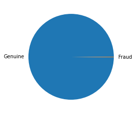
There is an imbalance in the data, with only 0.17% of the total cases being fraudulent.
Now we look at the distribution of the two named features in the dataset. For Time, it is clear that there was a particular duration in the day when most of the transactions took place:
# plot the named features
f, axes = plt.subplots(1, 2, figsize=(18,4), sharex = True)

amount_value = dataset['Amount'].values # values
time_value = dataset['Time'].values # values

sns.distplot(amount_value, hist=False, color="m", kde_kws={"shade": True}, ax=axes[0]).set_title('Distribution of Amount')
sns.distplot(time_value, hist=False, color="m", kde_kws={"shade": True}, ax=axes[1]).set_title('Distribution of Time')

plt.show()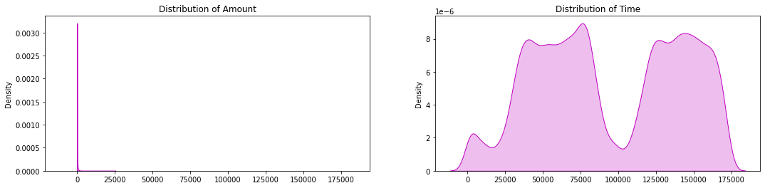
Let us check if there is any difference between valid transactions and fraudulent transactions:
print("Average Amount in a Fraudulent Transaction: " + str(dataset[dataset["Class"] == 1]["Amount"].mean()))
print("Average Amount in a Valid Transaction: " + str(dataset[dataset["Class"] == 0]["Amount"].mean()))
Average Amount in a Fraudulent Transaction: 122.21132113821133
Average Amount in a Valid Transaction: 88.29102242225574As we can notice from this, the average money transaction for the fraudulent ones is more. It makes this problem crucial to deal with. Now let us try to understand the distribution of values in each feature. Let's start with the Amount:
print("Summary of the feature - Amount" + "\n-------------------------------")
print(dataset["Amount"].describe())
Summary of the feature - Amount
-------------------------------
count 284807.000000
mean 88.349619
std 250.120109
min 0.000000
25% 5.600000
50% 22.000000
75% 77.165000
max 25691.160000
Name: Amount, dtype: float64The rest of the features don't have any physical interpretation and will be seen through histograms. Here the values are subgrouped according to class (valid or fraud):
# Reorder the columns Amount, Time then the rest
data_plot = dataset.copy()
amount = data_plot['Amount']
data_plot.drop(labels=['Amount'], axis=1, inplace = True)
data_plot.insert(0, 'Amount', amount)

# Plot the distributions of the features
columns = data_plot.iloc[:,0:30].columns
plt.figure(figsize=(12,30*4))
grids = gridspec.GridSpec(30, 1)
for grid, index in enumerate(data_plot[columns]):
 ax = plt.subplot(grids[grid])
 sns.distplot(data_plot[index][data_plot.Class == 1], hist=False, kde_kws={"shade": True}, bins=50)
 sns.distplot(data_plot[index][data_plot.Class == 0], hist=False, kde_kws={"shade": True}, bins=50)
 ax.set_xlabel("")
 ax.set_title("Distribution of Column: "  + str(index))
plt.show()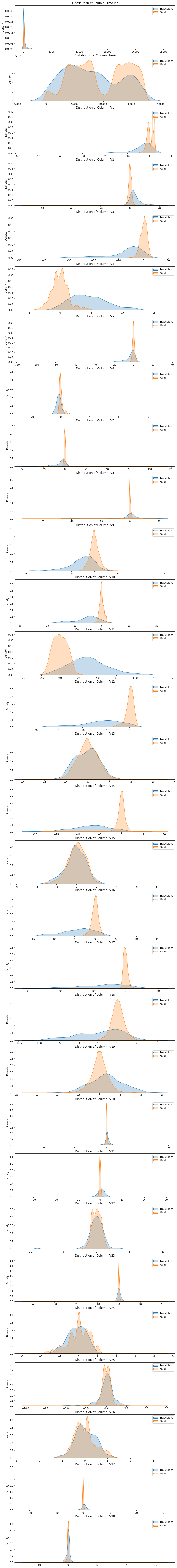
Data Preparation
Since the features are created using PCA, feature selection is unnecessary as many features are tiny. Let's see if there are any missing values in the dataset:
# check for null values
dataset.isnull().shape[0]
print("Non-missing values: " + str(dataset.isnull().shape[0]))
print("Missing values: " + str(dataset.shape[0] - dataset.isnull().shape[0]))
Non-missing values: 284807
Missing values: 0As there are no missing data, we turn to standardization. We standardize only Time and Amount using RobustScaler:
from sklearn.preprocessing import RobustScaler
scaler = RobustScaler().fit(dataset[["Time", "Amount"]])
dataset[["Time", "Amount"]] = scaler.transform(dataset[["Time", "Amount"]])

dataset.head().append(dataset.tail())
As we saw previously, the Amount column has outliers, that's why we chose RobustScaler() as it's robust to outliers. Output:
╔════════╤═══════════╤════════════╤═══════════╤═══════════╤═══════════╤═══════════╤═══════════╤═══════════╤═══════════╤═══════════╤═════╤═══════════╤═══════════╤═══════════╤═══════════╤═══════════╤═══════════╤═══════════╤═══════════╤═══════════╤═══════╗
║        │ Time      │ V1         │ V2        │ V3        │ V4        │ V5        │ V6        │ V7        │ V8        │ V9        │ ... │ V21       │ V22       │ V23       │ V24       │ V25       │ V26       │ V27       │ V28       │ Amount    │ Class ║
╠════════╪═══════════╪════════════╪═══════════╪═══════════╪═══════════╪═══════════╪═══════════╪═══════════╪═══════════╪═══════════╪═════╪═══════════╪═══════════╪═══════════╪═══════════╪═══════════╪═══════════╪═══════════╪═══════════╪═══════════╪═══════╣
║ 0      │ -0.994983 │ -1.359807  │ -0.072781 │ 2.536347  │ 1.378155  │ -0.338321 │ 0.462388  │ 0.239599  │ 0.098698  │ 0.363787  │ ... │ -0.018307 │ 0.277838  │ -0.110474 │ 0.066928  │ 0.128539  │ -0.189115 │ 0.133558  │ -0.021053 │ 1.783274  │ 0     ║
╟────────┼───────────┼────────────┼───────────┼───────────┼───────────┼───────────┼───────────┼───────────┼───────────┼───────────┼─────┼───────────┼───────────┼───────────┼───────────┼───────────┼───────────┼───────────┼───────────┼───────────┼───────╢
║ 1      │ -0.994983 │ 1.191857   │ 0.266151  │ 0.166480  │ 0.448154  │ 0.060018  │ -0.082361 │ -0.078803 │ 0.085102  │ -0.255425 │ ... │ -0.225775 │ -0.638672 │ 0.101288  │ -0.339846 │ 0.167170  │ 0.125895  │ -0.008983 │ 0.014724  │ -0.269825 │ 0     ║
╟────────┼───────────┼────────────┼───────────┼───────────┼───────────┼───────────┼───────────┼───────────┼───────────┼───────────┼─────┼───────────┼───────────┼───────────┼───────────┼───────────┼───────────┼───────────┼───────────┼───────────┼───────╢
║ 2      │ -0.994972 │ -1.358354  │ -1.340163 │ 1.773209  │ 0.379780  │ -0.503198 │ 1.800499  │ 0.791461  │ 0.247676  │ -1.514654 │ ... │ 0.247998  │ 0.771679  │ 0.909412  │ -0.689281 │ -0.327642 │ -0.139097 │ -0.055353 │ -0.059752 │ 4.983721  │ 0     ║
╟────────┼───────────┼────────────┼───────────┼───────────┼───────────┼───────────┼───────────┼───────────┼───────────┼───────────┼─────┼───────────┼───────────┼───────────┼───────────┼───────────┼───────────┼───────────┼───────────┼───────────┼───────╢
║ 3      │ -0.994972 │ -0.966272  │ -0.185226 │ 1.792993  │ -0.863291 │ -0.010309 │ 1.247203  │ 0.237609  │ 0.377436  │ -1.387024 │ ... │ -0.108300 │ 0.005274  │ -0.190321 │ -1.175575 │ 0.647376  │ -0.221929 │ 0.062723  │ 0.061458  │ 1.418291  │ 0     ║
╟────────┼───────────┼────────────┼───────────┼───────────┼───────────┼───────────┼───────────┼───────────┼───────────┼───────────┼─────┼───────────┼───────────┼───────────┼───────────┼───────────┼───────────┼───────────┼───────────┼───────────┼───────╢
║ 4      │ -0.994960 │ -1.158233  │ 0.877737  │ 1.548718  │ 0.403034  │ -0.407193 │ 0.095921  │ 0.592941  │ -0.270533 │ 0.817739  │ ... │ -0.009431 │ 0.798278  │ -0.137458 │ 0.141267  │ -0.206010 │ 0.502292  │ 0.219422  │ 0.215153  │ 0.670579  │ 0     ║
╟────────┼───────────┼────────────┼───────────┼───────────┼───────────┼───────────┼───────────┼───────────┼───────────┼───────────┼─────┼───────────┼───────────┼───────────┼───────────┼───────────┼───────────┼───────────┼───────────┼───────────┼───────╢
║ 284802 │ 1.034951  │ -11.881118 │ 10.071785 │ -9.834783 │ -2.066656 │ -5.364473 │ -2.606837 │ -4.918215 │ 7.305334  │ 1.914428  │ ... │ 0.213454  │ 0.111864  │ 1.014480  │ -0.509348 │ 1.436807  │ 0.250034  │ 0.943651  │ 0.823731  │ -0.296653 │ 0     ║
╟────────┼───────────┼────────────┼───────────┼───────────┼───────────┼───────────┼───────────┼───────────┼───────────┼───────────┼─────┼───────────┼───────────┼───────────┼───────────┼───────────┼───────────┼───────────┼───────────┼───────────┼───────╢
║ 284803 │ 1.034963  │ -0.732789  │ -0.055080 │ 2.035030  │ -0.738589 │ 0.868229  │ 1.058415  │ 0.024330  │ 0.294869  │ 0.584800  │ ... │ 0.214205  │ 0.924384  │ 0.012463  │ -1.016226 │ -0.606624 │ -0.395255 │ 0.068472  │ -0.053527 │ 0.038986  │ 0     ║
╟────────┼───────────┼────────────┼───────────┼───────────┼───────────┼───────────┼───────────┼───────────┼───────────┼───────────┼─────┼───────────┼───────────┼───────────┼───────────┼───────────┼───────────┼───────────┼───────────┼───────────┼───────╢
║ 284804 │ 1.034975  │ 1.919565   │ -0.301254 │ -3.249640 │ -0.557828 │ 2.630515  │ 3.031260  │ -0.296827 │ 0.708417  │ 0.432454  │ ... │ 0.232045  │ 0.578229  │ -0.037501 │ 0.640134  │ 0.265745  │ -0.087371 │ 0.004455  │ -0.026561 │ 0.641096  │ 0     ║
╟────────┼───────────┼────────────┼───────────┼───────────┼───────────┼───────────┼───────────┼───────────┼───────────┼───────────┼─────┼───────────┼───────────┼───────────┼───────────┼───────────┼───────────┼───────────┼───────────┼───────────┼───────╢
║ 284805 │ 1.034975  │ -0.240440  │ 0.530483  │ 0.702510  │ 0.689799  │ -0.377961 │ 0.623708  │ -0.686180 │ 0.679145  │ 0.392087  │ ... │ 0.265245  │ 0.800049  │ -0.163298 │ 0.123205  │ -0.569159 │ 0.546668  │ 0.108821  │ 0.104533  │ -0.167680 │ 0     ║
╟────────┼───────────┼────────────┼───────────┼───────────┼───────────┼───────────┼───────────┼───────────┼───────────┼───────────┼─────┼───────────┼───────────┼───────────┼───────────┼───────────┼───────────┼───────────┼───────────┼───────────┼───────╢
║ 284806 │ 1.035022  │ -0.533413  │ -0.189733 │ 0.703337  │ -0.506271 │ -0.012546 │ -0.649617 │ 1.577006  │ -0.414650 │ 0.486180  │ ... │ 0.261057  │ 0.643078  │ 0.376777  │ 0.008797  │ -0.473649 │ -0.818267 │ -0.002415 │ 0.013649  │ 2.724796  │ 0     ║
╚════════╧═══════════╧════════════╧═══════════╧═══════════╧═══════════╧═══════════╧═══════════╧═══════════╧═══════════╧═══════════╧═════╧═══════════╧═══════════╧═══════════╧═══════════╧═══════════╧═══════════╧═══════════╧═══════════╧═══════════╧═══════╝
10 rows × 31 columns
Next, let's divide the data into features and targets. We also make the train-test split of the data:
# Separate response and features  Undersampling before cross validation will lead to overfiting
y = dataset["Class"] # target
X = dataset.iloc[:,0:30]

# Use SKLEARN for the split
from sklearn.model_selection import train_test_split
X_train, X_test, y_train, y_test = train_test_split(
        X, y, test_size = 0.2, random_state = 42)

X_train.shape, X_test.shape, y_train.shape, y_test.shape
Output:
((227845, 30), (56962, 30), (227845,), (56962,))Let's import all the necessary libraries for the tutorial:
# Create the cross validation framework
from sklearn.model_selection import StratifiedKFold
from sklearn.model_selection import GridSearchCV, cross_val_score, RandomizedSearchCV

kf = StratifiedKFold(n_splits=5, random_state = None, shuffle = False)
# Import the imbalance Learn module
from imblearn.pipeline import make_pipeline ## Create a Pipeline using the provided estimators .
from imblearn.under_sampling import NearMiss ## perform Under-sampling based on NearMiss methods.
from imblearn.over_sampling import SMOTE ## PerformOver-sampling class that uses SMOTE.
# import the metrics
from sklearn.metrics import roc_curve, roc_auc_score, accuracy_score, recall_score, precision_score, f1_score
# Import the classifiers
from sklearn.linear_model import LogisticRegression
from sklearn.svm import SVC
from sklearn.neighbors import KNeighborsClassifier
from sklearn.tree import DecisionTreeClassifier
from sklearn.ensemble import RandomForestClassifierBuilding and Training the Model
Let's run RandomForestClassifier on the dataset and see the performance:
# Fit and predict
rfc = RandomForestClassifier()
rfc.fit(X_train, y_train)
y_pred = rfc.predict(X_test)

# For the performance let's use some metrics from SKLEARN module
from sklearn.metrics import accuracy_score, precision_score, recall_score, f1_score

print("The accuracy is", accuracy_score(y_test, y_pred))
print("The precision is", precision_score(y_test, y_pred))
print("The recall is", recall_score(y_test, y_pred))
print("The F1 score is", f1_score(y_test, y_pred))
The training should take a few minutes to finish. Here's the output:
The accuracy is 0.9996137776061234
The precision is 0.975
The recall is 0.7959183673469388
The F1 score is 0.8764044943820225
As you can see, we had only 0.17% fraud transactions, and a model predicting all transactions to be valid would have an accuracy of 99.83%. Luckily, our model exceeded that to over 99.96%.
As a result, accuracy isn't a suitable metric for our problem. There are three more:
- Precision: It is the total number of true positives divided by the true positives and false positives. Precision makes sure we don't spot good transactions as fraudulent in our problem.
- Recall: It is the total number of true positives divided by the true positives and false negatives. Recall assures we don't predict fraudulent transactions as all good and therefore get good accuracy with a terrible model.
- F1 Score: It is the harmonic mean of precision and recall. It makes a good average between both metrics.
The recall is more important than precision in our problem, as predicting a fraudulent transaction as good is worse than marking a good transaction as fraudulent, you can use fbeta_score() and adjust the beta parameter to make it more weighted towards recall.
In the upcoming sections, we will do a grid and randomized search on oversampling and undersampling on various classifiers.
Undersampling
In this section, we will perform undersampling to our dataset. One trivial point to note is that we will not undersample the testing data as we want our model to perform well with skewed class distributions.
The steps are as follows:
- Use a 5-fold cross-validation on the training set.
- On each of the folds, use undersampling.
- Fit the model on the training folds and validate on the validation fold.
NearMiss Methods
Imbalanced-Learn is a Python module that assists in balancing datasets that are strongly skewed or biased towards certain classes. It aids in resampling classes that are usually oversampled or undersampled. If the imbalance ratio is higher, the output is slanted toward the class with the most samples. Look at this tutorial to learn more about the imbalanced-learn module.
Near Miss refers to a group of undersampling strategies that pick samples based on the distance between majority and minority class instances.
In the below code, we're making a flexible function that can perform grid or randomized search on a given estimator and its parameters with or without under/oversampling and returns the best estimator along with the performance metrics:
def get_model_best_estimator_and_metrics(estimator, params, kf=kf, X_train=X_train,
                                         y_train=y_train, X_test=X_test,
                                         y_test=y_test, is_grid_search=True,
                                         sampling=NearMiss(), scoring="f1",
                                         n_jobs=2):
    if sampling is None:
        # make the pipeline of only the estimator, just so the remaining code will work fine
        pipeline = make_pipeline(estimator)
    else:
        # make the pipeline of over/undersampling and estimator
        pipeline = make_pipeline(sampling, estimator)
    # get the estimator name
    estimator_name = estimator.__class__.__name__.lower()
    # construct the parameters for grid/random search cv
    new_params = {f'{estimator_name}__{key}': params[key] for key in params}
    if is_grid_search:
        # grid search instead of randomized search
        search = GridSearchCV(pipeline, param_grid=new_params, cv=kf, return_train_score=True, n_jobs=n_jobs, verbose=2)
    else:
        # randomized search
        search = RandomizedSearchCV(pipeline, param_distributions=new_params,
                                    cv=kf, scoring=scoring, return_train_score=True,
                                    n_jobs=n_jobs, verbose=1)
    # fit the model
    search.fit(X_train, y_train)
    cv_score = cross_val_score(search, X_train, y_train, scoring=scoring, cv=kf)
    # make predictions on the test data
    y_pred = search.best_estimator_.named_steps[estimator_name].predict(X_test)
    # calculate the metrics: recall, accuracy, F1 score, etc.
    recall = recall_score(y_test, y_pred)
    accuracy = accuracy_score(y_test, y_pred)
    f1 = f1_score(y_test, y_pred)
    y_proba = search.best_estimator_.named_steps[estimator_name].predict_proba(X_test)[::, 1]
    fpr, tpr, _ = roc_curve(y_test, y_proba)
    auc = roc_auc_score(y_test, y_proba)
    # return the best estimator along with the metrics
    return {
        "best_estimator": search.best_estimator_,
        "estimator_name": estimator_name,
        "cv_score": cv_score,
        "recall": recall,
        "accuracy": accuracy,
        "f1_score": f1,
        "fpr": fpr,
        "tpr": tpr,
        "auc": auc,
    }
Because there is never enough data to train your model, eliminating a portion of it for validation causes underfitting. We risk losing crucial patterns/trends in the dataset by lowering the training data, which increases the error caused by bias. So, we need a strategy that offers enough data for training the model while simultaneously leaving enough data for validation.
The cross_val_score() function uses cross-validation to determine a score, which we're using in the above function. Check this tutorial to learn more about this function.
The function is made to be flexible. For example, if you want to perform a grid search on a LogisticRegression model with undersampling, you simply use this:
# Cumulatively create a table for the ROC curve
## Create the dataframe
res_table = pd.DataFrame(columns=['classifiers', 'fpr','tpr','auc'])

logreg_us_results = get_model_best_estimator_and_metrics(
    estimator=LogisticRegression(),
    params={"penalty": ['l1', 'l2'],
                  'C': [ 0.01, 0.1, 1, 100],
                  'solver' : ['liblinear']},
    sampling=NearMiss(),
)
print(f"==={logreg_us_results['estimator_name']}===")
print("Model:", logreg_us_results['best_estimator'])
print("Accuracy:", logreg_us_results['accuracy'])
print("Recall:", logreg_us_results['recall'])
print("F1 Score:", logreg_us_results['f1_score'])
res_table = res_table.append({'classifiers': logreg_us_results["estimator_name"],
                                        'fpr': logreg_us_results["fpr"],
                                        'tpr': logreg_us_results["tpr"],
                                        'auc': logreg_us_results["auc"]
                              }, ignore_index=True)
If you want to disable undersampling, you simply pass None to the sampling parameter on the get_model_best_estimator_and_metrics() function.
If you want to plot the ROC curve on multiple models, you can run the above code on numerous models and their parameters. Just make sure to edit the classifier name to distinguish between oversampled and undersampled models.
I have managed to run five different models on undersampling (took a lot of hours to train), and here's how we plot our ROC curve using our res_table:
# Plot the ROC curve for undersampling
res_table.set_index('classifiers', inplace=True)
fig = plt.figure(figsize=(17,7))

for j in res_table.index:
    plt.plot(res_table.loc[j]['fpr'],
             res_table.loc[j]['tpr'],
             label="{}, AUC={:.3f}".format(j, res_table.loc[j]['auc']))

plt.plot([0,1], [0,1], color='orange', linestyle='--')
plt.xticks(np.arange(0.0, 1.1, step=0.1))
plt.xlabel("Positive Rate(False)", fontsize=15)
plt.yticks(np.arange(0.0, 1.1, step=0.1))
plt.ylabel("Positive Rate(True)", fontsize=15)
plt.title('Analysis for Oversampling', fontweight='bold', fontsize=15)
plt.legend(prop={'size':13}, loc='lower right')
plt.show()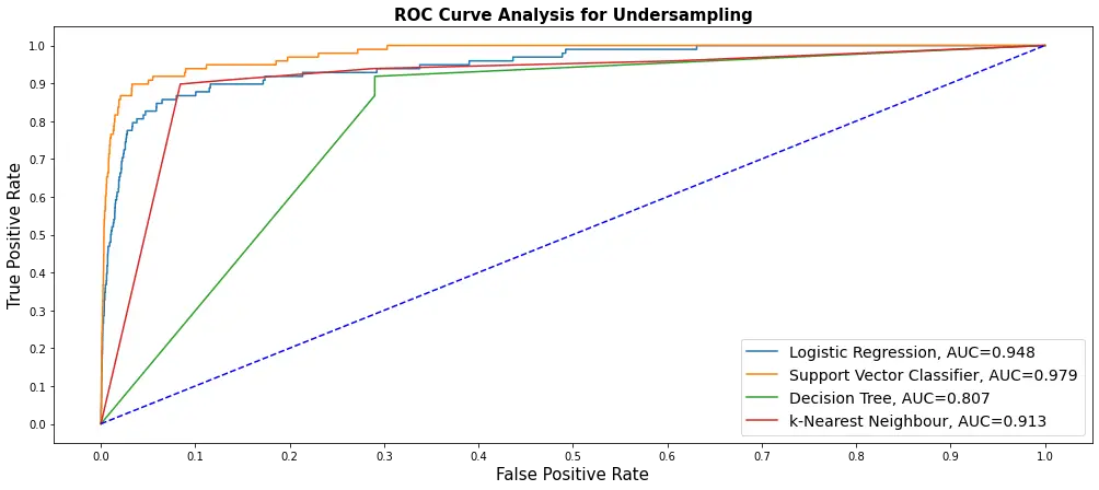
These were trained using NearMiss() undersampling and on five different models. So, if you run the above code, you'll see only one curve for LogisticRegression; make sure you copy that cell and do it for other models if you want.
Oversampling with SMOTE
One issue with unbalanced classification is that there are too few samples of the minority class for a model to learn the decision boundary successfully. Oversampling instances from the minority class is one solution to the issue. Before fitting a model, we duplicate samples from the minority class in the training set.
Synthesizing new instances from the minority class is an improvement over replicating examples from the minority class. It is a particularly efficient type of data augmentation for tabular data. This paper demonstrates that a combination of oversampling the minority class and undersampling the majority class may improve the classifier performance.
Similarly, you can pass SMOTE() to the sampling parameter on our function for oversampling:
# Cumulatively create a table for the ROC curve
res_table = pd.DataFrame(columns=['classifiers', 'fpr','tpr','auc'])

lin_reg_os_results = get_model_best_estimator_and_metrics(
    estimator=LogisticRegression(),
    params={"penalty": ['l1', 'l2'], 'C': [ 0.01, 0.1, 1, 100, 100],
            'solver' : ['liblinear']},
    sampling=SMOTE(random_state=42),
    scoring="f1",
    is_grid_search=False,
    n_jobs=2,
)
print(f"==={lin_reg_os_results['estimator_name']}===")
print("Model:", lin_reg_os_results['best_estimator'])
print("Accuracy:", lin_reg_os_results['accuracy'])
print("Recall:", lin_reg_os_results['recall'])
print("F1 Score:", lin_reg_os_results['f1_score'])
res_table = res_table.append({'classifiers': lin_reg_os_results["estimator_name"],
                                        'fpr': lin_reg_os_results["fpr"],
                                        'tpr': lin_reg_os_results["tpr"],
                                        'auc': lin_reg_os_results["auc"]
                              }, ignore_index=True)
Notice we set is_grid_search to False as we know this will take a very long time, so we use RandomizedSearchCV. Consider increasing n_jobs to more than two if you have a higher number of cores (Currently, a Google Colab instance has only 2 CPU cores).
Appendix: Outlier Detection and Removal
The outlier presence sometimes affects the model and might lead us to wrong conclusions. Therefore, we must look at the data distribution while keeping a close eye on the outliers. This section of this tutorial uses the Interquartile Range (IQR) method to identify and remove the outliers:
# boxplot for two example variables in the dataset

f, axes = plt.subplots(1, 2, figsize=(18,4), sharex = True)

variable1 = dataset["V1"]
variable2 = dataset["V2"]

sns.boxplot(variable1, color="m", ax=axes[0]).set_title('Boxplot for V1')
sns.boxplot(variable2, color="m", ax=axes[1]).set_title('Boxplot for V2')

plt.show()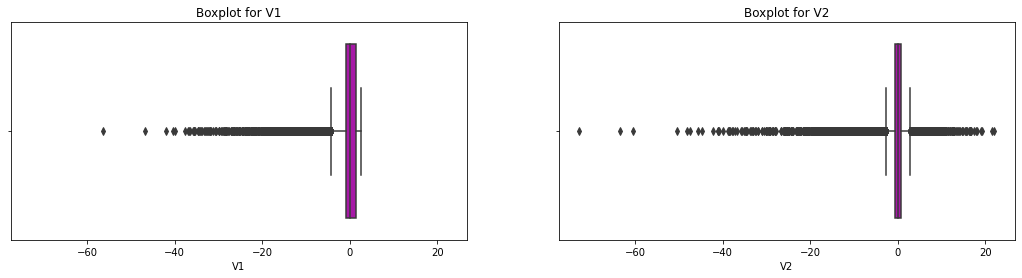
Getting the range:
# Find the IQR for all the feature variables
# Please note that we are keeping Class variable also in this evaluation, though we know using this method no observation
# be removed based on this variable.

quartile1 = dataset.quantile(0.25)
quartile3 = dataset.quantile(0.75)

IQR = quartile3 - quartile1
print(IQR)
Time 1.000000
V1 2.236015
V2 1.402274
V3 1.917560
V4 1.591981
V5 1.303524
V6 1.166861
V7 1.124512
V8 0.535976
V9 1.240237
V10 0.989349
V11 1.502088
V12 1.023810
V13 1.311044
V14 0.918724
V15 1.231705
V16 0.991333
V17 0.883423
V18 0.999657
V19 0.915248
V20 0.344762
V21 0.414772
V22 1.070904
V23 0.309488
V24 0.794113
V25 0.667861
V26 0.567936
V27 0.161885
V28 0.131240
Amount 1.000000
Class 0.000000
dtype: float64Now that we have the Interquartile range for each variable, we remove the observations with outlier values. We have used "outlier constant" to be 3:
# Remove the outliers
constant = 3
datavalid = dataset[~((dataset < (quartile1 - constant * IQR)) |(dataset > (quartile3 + constant * IQR))).any(axis=1)]
deletedrows = dataset.shape[0] - datavalid.shape[0]
print("We have removed " + str(deletedrows) + " rows from the data as outliers")
Output:
We have removed 53376 rows from the data as outliersConclusion
This tutorial trained different classifiers and performed undersampling and oversampling techniques after splitting the data into training and test sets to decide which classifier is more effective in detecting fraudulent transactions.
GridSearchCV takes a lot of time and is therefore only effective in undersampling since undersampling does not take much time during training. If you find it's taking forever on a particular model, consider reducing the parameters you've passed, and use RandomizedSearchCV for that (i.e., setting is_grid_search to False on our core function).
If you see that searching for optimal parameters takes time (and it does), consider directly using the RandomForestClassifier model, as it's relatively faster to train and usually does not overfit or underfit, as you saw earlier in the tutorial.
The SMOTE algorithm creates new synthetic points from the minority class to achieve a quantitative balance with the majority class. Although SMOTE may be more accurate than random undersampling, it does not delete any rows but will spend more time on training.
It will help if you do not oversample or undersample your data before cross-validation because you are directly impacting the validation set by oversampling or undersampling before using cross-validation, resulting in the data leakage issue.
You can get the complete code here.
Learn also: Imbalance Learning with Imblearn and Smote Variants Libraries in Python
Happy learning ♥
Liked what you read? You'll love what you can learn from our AI-powered Code Explainer. Check it out!
View Full Code Generate Python Code


Got a coding query or need some guidance before you comment? Check out this Python Code Assistant for expert advice and handy tips. It's like having a coding tutor right in your fingertips!