Want to code faster? Our Python Code Generator lets you create Python scripts with just a few clicks. Try it now!
![]()
Skin cancer is an abnormal growth of skin cells, it is one of the most common cancers and unfortunately, it can become deadly. The good news though is when caught early, your dermatologist can treat it and eliminate it entirely.
Using deep learning and neural networks, we'll be able to classify benign and malignant skin diseases, which may help the doctor diagnose cancer at an earlier stage. In this tutorial, we will make a skin disease classifier that tries to distinguish between benign (nevus and seborrheic keratosis) and malignant (melanoma) skin diseases from only photographic images using TensorFlow framework in Python.
To get started, let's install the required libraries:
pip3 install tensorflow tensorflow_hub matplotlib seaborn numpy pandas sklearn imblearn
Open up a new notebook (or Google Colab) and import the necessary modules:
import tensorflow as tf
import tensorflow_hub as hub
import matplotlib.pyplot as plt
import numpy as np
import pandas as pd
import seaborn as sns
from tensorflow.keras.utils import get_file
from sklearn.metrics import roc_curve, auc, confusion_matrix
from imblearn.metrics import sensitivity_score, specificity_score

import os
import glob
import zipfile
import random

# to get consistent results after multiple runs
tf.random.set_seed(7)
np.random.seed(7)
random.seed(7)

# 0 for benign, 1 for malignant
class_names = ["benign", "malignant"]
Related: Image Captioning using PyTorch and Transformers in Python.
Preparing the Dataset
For this tutorial, we'll be using only a small part of ISIC archive dataset, the below function downloads and extract the dataset into a new data folder:
def download_and_extract_dataset():
  # dataset from https://github.com/udacity/dermatologist-ai
  # 5.3GB
  train_url = "https://s3-us-west-1.amazonaws.com/udacity-dlnfd/datasets/skin-cancer/train.zip"
  # 824.5MB
  valid_url = "https://s3-us-west-1.amazonaws.com/udacity-dlnfd/datasets/skin-cancer/valid.zip"
  # 5.1GB
  test_url  = "https://s3-us-west-1.amazonaws.com/udacity-dlnfd/datasets/skin-cancer/test.zip"
  for i, download_link in enumerate([valid_url, train_url, test_url]):
    temp_file = f"temp{i}.zip"
    data_dir = get_file(origin=download_link, fname=os.path.join(os.getcwd(), temp_file))
    print("Extracting", download_link)
    with zipfile.ZipFile(data_dir, "r") as z:
      z.extractall("data")
    # remove the temp file
    os.remove(temp_file)

# comment the below line if you already downloaded the dataset
download_and_extract_dataset()
This will take several minutes depending on your connection, after that, the data folder will appear that contains the training, validation and testing sets. Each set is a folder that has three categories of skin disease images (nevus, seborrheic_keratosis and melanoma).
Note: You may struggle to download the dataset using the above Python function when you have a slow Internet connection, in that case, you should download it and extract it manually in the folder data in the current directory.
Now that we have the dataset in our machine, let's find a way to label these images, remember we're going to classify only benign and malignant skin diseases, so we need to label nevus and seborrheic keratosis as the value 0 and melanoma 1.
The below cell generates a metadata CSV file for each set, each row in the CSV file corresponds to a path to an image along with its label (0 or 1):
# preparing data
# generate CSV metadata file to read img paths and labels from it
def generate_csv(folder, label2int):
    folder_name = os.path.basename(folder)
    labels = list(label2int)
    # generate CSV file
    df = pd.DataFrame(columns=["filepath", "label"])
    i = 0
    for label in labels:
        print("Reading", os.path.join(folder, label, "*"))
        for filepath in glob.glob(os.path.join(folder, label, "*")):
            df.loc[i] = [filepath, label2int[label]]
            i += 1
    output_file = f"{folder_name}.csv"
    print("Saving", output_file)
    df.to_csv(output_file)

# generate CSV files for all data portions, labeling nevus and seborrheic keratosis
# as 0 (benign), and melanoma as 1 (malignant)
# you should replace "data" path to your extracted dataset path
# don't replace if you used download_and_extract_dataset() function
generate_csv("data/train", {"nevus": 0, "seborrheic_keratosis": 0, "melanoma": 1})
generate_csv("data/valid", {"nevus": 0, "seborrheic_keratosis": 0, "melanoma": 1})
generate_csv("data/test", {"nevus": 0, "seborrheic_keratosis": 0, "melanoma": 1})
The generate_csv() function accepts 2 arguments, the first is the path of the set, for example, if you have downloaded and extract the dataset in "E:\datasets\skin-cancer", then the training set should be something like "E:\datasets\skin-cancer\train".
The second parameter is a dictionary that maps each skin disease category to its corresponding label value (again, 0 for benign and 1 for malignant).
The reason I did a function like this is the ability to use it on other skin disease classifications (such as melanocytic classification), so you can add more skin diseases and use it for other problems as well.
Once you run the cell, you notice that 3 CSV files will appear in your current directory. Now let's use the from_tensor_slices() method from tf.data API to load these metadata files:
# loading data
train_metadata_filename = "train.csv"
valid_metadata_filename = "valid.csv"
# load CSV files as DataFrames
df_train = pd.read_csv(train_metadata_filename)
df_valid = pd.read_csv(valid_metadata_filename)
n_training_samples = len(df_train)
n_validation_samples = len(df_valid)
print("Number of training samples:", n_training_samples)
print("Number of validation samples:", n_validation_samples)
train_ds = tf.data.Dataset.from_tensor_slices((df_train["filepath"], df_train["label"]))
valid_ds = tf.data.Dataset.from_tensor_slices((df_valid["filepath"], df_valid["label"]))
Now we have loaded the dataset (train_ds and valid_ds), each sample is a tuple of filepath (path to the image file) and label (0 for benign and 1 for malignant), here is the output:
Number of training samples: 2000
Number of validation samples: 150
Let's load the images:
# preprocess data
def decode_img(img):
  # convert the compressed string to a 3D uint8 tensor
  img = tf.image.decode_jpeg(img, channels=3)
  # Use `convert_image_dtype` to convert to floats in the [0,1] range.
  img = tf.image.convert_image_dtype(img, tf.float32)
  # resize the image to the desired size.
  return tf.image.resize(img, [299, 299])


def process_path(filepath, label):
  # load the raw data from the file as a string
  img = tf.io.read_file(filepath)
  img = decode_img(img)
  return img, label


valid_ds = valid_ds.map(process_path)
train_ds = train_ds.map(process_path)
# test_ds = test_ds
for image, label in train_ds.take(1):
    print("Image shape:", image.shape)
    print("Label:", label.numpy())
The above code uses map() method to execute process_path() function on each sample on both sets, it'll basically load the images, decode the image format, convert the image pixels to be in the range [0, 1] and resize it to (299, 299, 3), we then take one image and print its shape:
Image shape: (299, 299, 3)
Label: 0
Everything is as expected, now let's prepare this dataset for training:
# training parameters
batch_size = 64
optimizer = "rmsprop"

def prepare_for_training(ds, cache=True, batch_size=64, shuffle_buffer_size=1000):
  if cache:
    if isinstance(cache, str):
      ds = ds.cache(cache)
    else:
      ds = ds.cache()
  # shuffle the dataset
  ds = ds.shuffle(buffer_size=shuffle_buffer_size)
  # Repeat forever
  ds = ds.repeat()
  # split to batches
  ds = ds.batch(batch_size)
  # `prefetch` lets the dataset fetch batches in the background while the model
  # is training.
  ds = ds.prefetch(buffer_size=tf.data.experimental.AUTOTUNE)
  return ds

valid_ds = prepare_for_training(valid_ds, batch_size=batch_size, cache="valid-cached-data")
train_ds = prepare_for_training(train_ds, batch_size=batch_size, cache="train-cached-data")
Here is what we did:
cache(): Since we're making too many calculations on each set, we usedcache()method to save our preprocessed dataset into a local cache file, this will only preprocess it the very first time (in the first epoch during training).shuffle(): To basically shuffle the dataset, so the samples are in random order.repeat(): Every time we iterate over the dataset, it'll keep generating samples for us repeatedly, this will help us during the training.batch(): We batch our dataset into 64 or 32 samples per training step.prefetch(): This will enable us to fetch batches in the background while the model is training.
The below cell gets the first validation batch and plots the images along with their corresponding label:
batch = next(iter(valid_ds))

def show_batch(batch):
  plt.figure(figsize=(12,12))
  for n in range(25):
      ax = plt.subplot(5,5,n+1)
      plt.imshow(batch[0][n])
      plt.title(class_names[batch[1][n].numpy()].title())
      plt.axis('off')

show_batch(batch)
Output:
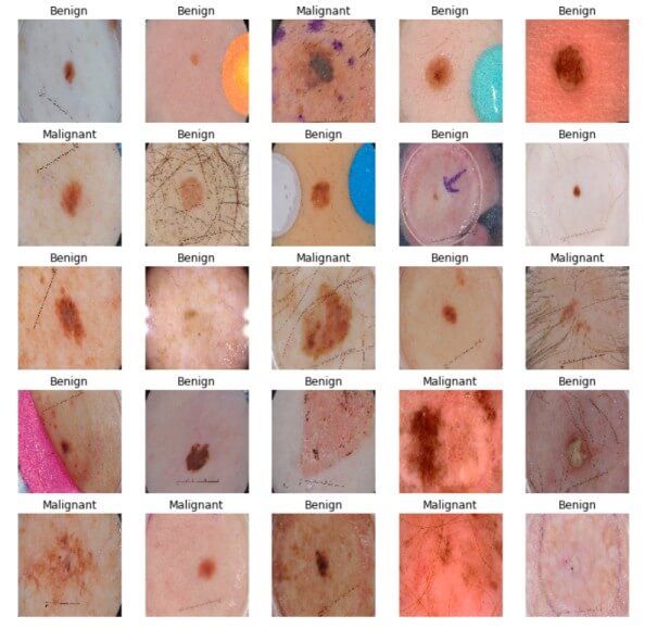
As you can see, it's extremely hard to differentiate between malignant and benign diseases, let's see how our model will deal with it.
Great, now our dataset is ready, let's dive into building our model.
Building the Model
Notice before, we resized all images to (299, 299, 3), and that's because of what InceptionV3 architecture expects as input, so we'll be using transfer learning with TensorFlow Hub library to download and load the InceptionV3 architecture along with its ImageNet pre-trained weights:
# building the model
# InceptionV3 model & pre-trained weights
module_url = "https://tfhub.dev/google/tf2-preview/inception_v3/feature_vector/4"
m = tf.keras.Sequential([
    hub.KerasLayer(module_url, output_shape=[2048], trainable=False),
    tf.keras.layers.Dense(1, activation="sigmoid")
])

m.build([None, 299, 299, 3])
m.compile(loss="binary_crossentropy", optimizer=optimizer, metrics=["accuracy"])
m.summary()
We set trainable to False so we won't be able to adjust the pre-trained weights during our training, we also added a final output layer with 1 unit that is expected to output a value between 0 and 1 (close to 0 means benign, and 1 for malignant).
After that, since this is a binary classification, we built our model using binary crossentropy loss, and used accuracy as our metric (not that reliable metric, we'll see sooner why), here is the output of our model summary:
Model: "sequential"
_________________________________________________________________
Layer (type)                 Output Shape              Param #
=================================================================
keras_layer (KerasLayer)     multiple                  21802784
_________________________________________________________________
dense (Dense)                multiple                  2049
=================================================================
Total params: 21,804,833
Trainable params: 2,049
Non-trainable params: 21,802,784
_________________________________________________________________
Learn also: Satellite Image Classification using TensorFlow in Python
Training the Model
We now have our dataset and the model, let's get them together:
model_name = f"benign-vs-malignant_{batch_size}_{optimizer}"
tensorboard = tf.keras.callbacks.TensorBoard(log_dir=os.path.join("logs", model_name))
# saves model checkpoint whenever we reach better weights
modelcheckpoint = tf.keras.callbacks.ModelCheckpoint(model_name + "_{val_loss:.3f}.h5", save_best_only=True, verbose=1)

history = m.fit(train_ds, validation_data=valid_ds,
                steps_per_epoch=n_training_samples // batch_size,
                validation_steps=n_validation_samples // batch_size, verbose=1, epochs=100,
                callbacks=[tensorboard, modelcheckpoint])
We're using ModelCheckpoint callback to save the best weights so far on each epoch, that's why I set epochs to 100, that's because it can converge to better weights at any time, to save your time, feel free to reduce that to 30 or so.
I also added tensorboard as a callback in case you want to experiment with different hyperparameter values.
Since fit() method doesn't know the number of samples there are in the dataset, we need to specify steps_per_epoch and validation_steps parameters for the number of iterations (the number of samples divided by the batch size) of the training set and validation set respectively.
Here is a part of the output during training:
Train for 31 steps, validate for 2 steps
Epoch 1/100
30/31 [============================>.] - ETA: 9s - loss: 0.4609 - accuracy: 0.7760
Epoch 00001: val_loss improved from inf to 0.49703, saving model to benign-vs-malignant_64_rmsprop_0.497.h5
31/31 [==============================] - 282s 9s/step - loss: 0.4646 - accuracy: 0.7722 - val_loss: 0.4970 - val_accuracy: 0.8125
<..SNIPED..>
Epoch 27/100
30/31 [============================>.] - ETA: 0s - loss: 0.2982 - accuracy: 0.8708
Epoch 00027: val_loss improved from 0.40253 to 0.38991, saving model to benign-vs-malignant_64_rmsprop_0.390.h5
31/31 [==============================] - 21s 691ms/step - loss: 0.3025 - accuracy: 0.8684 - val_loss: 0.3899 - val_accuracy: 0.8359
<..SNIPED..>
Epoch 41/100
30/31 [============================>.] - ETA: 0s - loss: 0.2800 - accuracy: 0.8802
Epoch 00041: val_loss did not improve from 0.38991
31/31 [==============================] - 21s 690ms/step - loss: 0.2829 - accuracy: 0.8790 - val_loss: 0.3948 - val_accuracy: 0.8281
Epoch 42/100
30/31 [============================>.] - ETA: 0s - loss: 0.2680 - accuracy: 0.8859
Epoch 00042: val_loss did not improve from 0.38991
31/31 [==============================] - 21s 693ms/step - loss: 0.2722 - accuracy: 0.8831 - val_loss: 0.4572 - val_accuracy: 0.8047
Model Evaluation
First, let's load our test set, just like previously:
# evaluation
# load testing set
test_metadata_filename = "test.csv"
df_test = pd.read_csv(test_metadata_filename)
n_testing_samples = len(df_test)
print("Number of testing samples:", n_testing_samples)
test_ds = tf.data.Dataset.from_tensor_slices((df_test["filepath"], df_test["label"]))

def prepare_for_testing(ds, cache=True, shuffle_buffer_size=1000):
  if cache:
    if isinstance(cache, str):
      ds = ds.cache(cache)
    else:
      ds = ds.cache()
  ds = ds.shuffle(buffer_size=shuffle_buffer_size)
  return ds

test_ds = test_ds.map(process_path)
test_ds = prepare_for_testing(test_ds, cache="test-cached-data")
The above code loads our test data and prepares it for testing:
Number of testing samples: 600600 images of the shape (299, 299, 3) can fit our memory, let's convert our test set from tf.data into a NumPy array:
# convert testing set to numpy array to fit in memory (don't do that when testing
# set is too large)
y_test = np.zeros((n_testing_samples,))
X_test = np.zeros((n_testing_samples, 299, 299, 3))
for i, (img, label) in enumerate(test_ds.take(n_testing_samples)):
  # print(img.shape, label.shape)
  X_test[i] = img
  y_test[i] = label.numpy()

print("y_test.shape:", y_test.shape)
The above cell will construct our arrays, it will take some time the first time it's executed because it's doing all the preprocessing defined in process_path() and prepare_for_testing() functions.
Now let's load our optimal weights that were saved by ModelCheckpoint during the training:
# load the weights with the least loss
m.load_weights("benign-vs-malignant_64_rmsprop_0.390.h5")
You may not have the exact filename of the optimal weights, you need to search for the saved weights in the current directory that has the least loss, the below code evaluates the model using the accuracy metric:
print("Evaluating the model...")
loss, accuracy = m.evaluate(X_test, y_test, verbose=0)
print("Loss:", loss, "  Accuracy:", accuracy)
Output:
Evaluating the model...
Loss: 0.4476394319534302   Accuracy: 0.8
We've reached about 84% accuracy on the validation set and 80% on the test set, but that's not all. Since our dataset is largely unbalanced, accuracy doesn't tell everything. In fact, a model that predicts every image as benign would get an accuracy of 80%, since malignant samples are about 20% of the total validation set.
As a result, we need a better way to evaluate our model, in the upcoming cells, we'll use seaborn and matplotlib libraries to draw the confusion matrix that tells us more about how well our model is doing.
But before we do that, I just want to make something clear: we all know that predicting a malignant disease as benign is a terrible mistake, you can kill people doing that! So we need a way to predict even more malignant cases even though we have very few malignant samples compared to benign ones. A good method is introducing a threshold.
Remember the output of the neural network is a value between 0 and 1. In the normal way, when the neural network produces a value between 0 and 0.5, we automatically assign it as benign, and from 0.5 to 1.0 as malignant. And since we want to be aware of the fact that we can predict a malignant disease as benign (that's only one of the many reasons), we can say for example, from 0 to 0.3 is benign, and from 0.3 to 1.0 is malignant, this means we are using a threshold value of 0.3, this will improve our predictions.
The below function does that:
def get_predictions(threshold=None):
  """
  Returns predictions for binary classification given `threshold`
  For instance, if threshold is 0.3, then it'll output 1 (malignant) for that sample if
  the probability of 1 is 30% or more (instead of 50%)
  """
  y_pred = m.predict(X_test)
  if not threshold:
    threshold = 0.5
  result = np.zeros((n_testing_samples,))
  for i in range(n_testing_samples):
    # test melanoma probability
    if y_pred[i][0] >= threshold:
      result[i] = 1
    # else, it's 0 (benign)
  return result

threshold = 0.23
# get predictions with 23% threshold
# which means if the model is 23% sure or more that is malignant,
# it's assigned as malignant, otherwise it's benign
y_pred = get_predictions(threshold)
accuracy_after = accuracy_score(y_test, y_pred)
print("Accuracy after setting the threshold:", accuracy_after)
Output:
19/19 [==============================] - 2s 123ms/step
Accuracy after setting the threshold: 0.7883333333333333
Now let's draw our confusion matrix and interpret it:
def plot_confusion_matrix(y_test, y_pred):
  cmn = confusion_matrix(y_test, y_pred)
  # Normalise
  cmn = cmn.astype('float') / cmn.sum(axis=1)[:, np.newaxis]
  # print it
  print(cmn)
  fig, ax = plt.subplots(figsize=(10,10))
  sns.heatmap(cmn, annot=True, fmt='.2f',
              xticklabels=[f"pred_{c}" for c in class_names],
              yticklabels=[f"true_{c}" for c in class_names],
              cmap="Blues"
              )
  plt.ylabel('Actual')
  plt.xlabel('Predicted')
  # plot the resulting confusion matrix
  plt.show()

plot_confusion_matrix(y_test, y_pred)
Output:
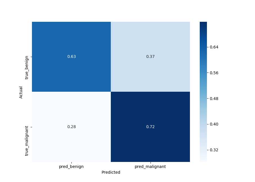
Sensitivity
So our model gets about 0.72 probability of a positive test given that the patient has the disease (bottom right of the confusion matrix), that's often called sensitivity.
Sensitivity is a statistical measure that is widely used in medicine that is given by the following formula (from Wikipedia):

72% of them as malignant, not bad but needs improvements.
Specificity
The other metric is specificity, you can read it in the top left of the confusion matrix, we got about 63%. It is basically the probability of a negative test given that the patient is well:

63% of them as benign.
With high specificity, the test rarely gives positive results in healthy patients, whereas a high sensitivity means that the model is reliable when its result is negative, I invite you to read more about it in this Wikipedia article.
Alternatively, you can use imblearn module to get these scores:
sensitivity = sensitivity_score(y_test, y_pred)
specificity = specificity_score(y_test, y_pred)

print("Melanoma Sensitivity:", sensitivity)
print("Melanoma Specificity:", specificity)
Output:
Melanoma Sensitivity: 0.717948717948718
Melanoma Specificity: 0.6252587991718427
Receiver Operating Characteristic
Another good metric is ROC, which is basically a graphical plot that shows us the diagnostic ability of our binary classifier, it features a true positive rate on the Y-axis and a false-positive rate on the X-axis. The perfect point we want to reach is in the top left corner of the plot, here is the code for plotting the ROC curve using matplotlib:
def plot_roc_auc(y_true, y_pred):
    """
    This function plots the ROC curves and provides the scores.
    """
    # prepare for figure
    plt.figure()
    fpr, tpr, _ = roc_curve(y_true, y_pred)
    # obtain ROC AUC
    roc_auc = auc(fpr, tpr)
    # print score
    print(f"ROC AUC: {roc_auc:.3f}")
    # plot ROC curve
    plt.plot(fpr, tpr, color="blue", lw=2,
                label='ROC curve (area = {f:.2f})'.format(d=1, f=roc_auc))
    plt.xlim([0.0, 1.0])
    plt.ylim([0.0, 1.05])
    plt.xlabel('False Positive Rate')
    plt.ylabel('True Positive Rate')
    plt.title('ROC curves')
    plt.legend(loc="lower right")
    plt.show()

plot_roc_auc(y_test, y_pred)
Output:
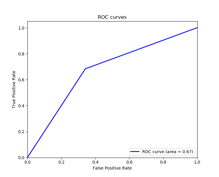
ROC AUC: 0.671Awesome, since we want to maximize the true positive rate, and minimize the false positive rate, calculating the area underneath the ROC curve proves to be useful, we got 0.671 as the Area Under Curve ROC (ROC AUC), an area of 1 means the model is ideal for all cases.
Predicting the Class of Images
Now that we're sure that our model is relatively good at predicting the benign and malignant classes after tweaking the hyperparameters or changing the model. Let's make a function that predicts the class of any image passed to it:
# a function given a function, it predicts the class of the image
def predict_image_class(img_path, model, threshold=0.5):
  img = tf.keras.preprocessing.image.load_img(img_path, target_size=(299, 299))
  img = tf.keras.preprocessing.image.img_to_array(img)
  img = tf.expand_dims(img, 0) # Create a batch
  img = tf.keras.applications.inception_v3.preprocess_input(img)
  img = tf.image.convert_image_dtype(img, tf.float32)
  predictions = model.predict(img)
  score = predictions.squeeze()
  if score >= threshold:
    print(f"This image is {100 * score:.2f}% malignant.")
  else:
    print(f"This image is {100 * (1 - score):.2f}% benign.")
  plt.imshow(img[0])
  plt.axis('off')
  plt.show()
Great. Let's pick a random image of each class from the test set. Starting with melanoma:
predict_image_class("data/test/melanoma/ISIC_0013767.jpg", m)Output:
This image is 68.04% malignant. Now a random nevus image:
predict_image_class("data/test/nevus/ISIC_0012092.jpg", m)Output:
This image is 78.41% benign. A random seborrheic keratosis one:
predict_image_class("data/test/seborrheic_keratosis/ISIC_0012136.jpg", m)Output:
This image is 86.32% benign.
Conclusion
We're done! There you have it, see how you can improve the model, we only used 2000 training samples, go to ISIC archive and download more and add them to the data folder, the scores will improve significantly depending on the number of samples you add. You can use ISIC archive downloader which may help you download the dataset in the way you want.
I also encourage you to tweak the hyperparameters such as the threshold we set earlier, and see if you can get better sensitivity and specificity scores.
I used InceptionV3 model architecture, you're free to use any CNN architecture you want, I invite you to browse TensorFlow hub and choose the newest model. For example, in satellite image classification, we've chosen EfficientNET V2, try it out and you may increase the performance significantly!
You can check out the complete code or Colab notebook.
References
Learn also: How to Perform YOLO Object Detection using OpenCV and PyTorch in Python.
![]()
Happy Learning ♥
Just finished the article? Now, boost your next project with our Python Code Generator. Discover a faster, smarter way to code.
View Full Code Explain The Code for Me


Got a coding query or need some guidance before you comment? Check out this Python Code Assistant for expert advice and handy tips. It's like having a coding tutor right in your fingertips!