Struggling with multiple programming languages? No worries. Our Code Converter has got you covered. Give it a go!
![]()
Satellite image classification is undoubtedly crucial for many applications in agriculture, environmental monitoring, urban planning, and more. Applications such as crop monitoring, land and forest cover mapping are emerging to be utilized by governments and companies, and labs for real-world use.
In this tutorial, you will learn how to build a satellite image classifier using the TensorFlow framework in Python.
We will be using the EuroSAT dataset based on Sentinel-2 satellite images covering 13 spectral bands. It consists of 27,000 labeled samples of 10 different classes: annual and permanent crop, forest, herbaceous vegetation, highway, industrial, pasture, residential, river, and sea lake.
EuroSAT dataset comes in two varieties:
rgb(default) with RGB that contain only the R, G, B frequency bands encoded as JPEG images.all: contains all 13 bands in the original value range.
Related: Image Captioning using PyTorch and Transformers in Python.
Getting Started
To get started, let's install TensorFlow and some other helper tools:
$ pip install tensorflow tensorflow_addons tensorflow_datasets tensorflow_hub numpy matplotlib seaborn sklearnWe use tensorflow_addons to calculate the F1 score during the training of the model.
We will use the EfficientNetV2 model which is the current state of the art on most image classification tasks. We use tensorflow_hub to load this pre-trained CNN model for fine-tuning.
Preparing the Dataset
Importing the necessary libraries:
import os

import numpy as np
import matplotlib.pyplot as plt
import seaborn as sns
import tensorflow as tf
import tensorflow_datasets as tfds
import tensorflow_hub as hub
import tensorflow_addons as tfa
Downloading and loading the dataset:
# load the whole dataset, for data info
all_ds   = tfds.load("eurosat", with_info=True)
# load training, testing & validation sets, splitting by 60%, 20% and 20% respectively
train_ds = tfds.load("eurosat", split="train[:60%]")
test_ds  = tfds.load("eurosat", split="train[60%:80%]")
valid_ds = tfds.load("eurosat", split="train[80%:]")
We split our dataset into 60% training, 20% validation during training, and 20% for testing. The below code is responsible for setting some variables we use for later:
# the class names
class_names = all_ds[1].features["label"].names
# total number of classes (10)
num_classes = len(class_names)
num_examples = all_ds[1].splits["train"].num_examples
We grab the list of classes from the all_ds dataset as it was loaded with with_info set to True, we also get the number of samples from it.
Next, I'm going to make a bar plot to see the number of samples in each class:
# make a plot for number of samples on each class
fig, ax = plt.subplots(1, 1, figsize=(14,10))
labels, counts = np.unique(np.fromiter(all_ds[0]["train"].map(lambda x: x["label"]), np.int32),
                       return_counts=True)

plt.ylabel('Counts')
plt.xlabel('Labels')
sns.barplot(x = [class_names[l] for l in labels], y = counts, ax=ax)
for i, x_ in enumerate(labels):
  ax.text(x_-0.2, counts[i]+5, counts[i])
# set the title
ax.set_title("Bar Plot showing Number of Samples on Each Class")
# save the image
# plt.savefig("class_samples.png")
Output:
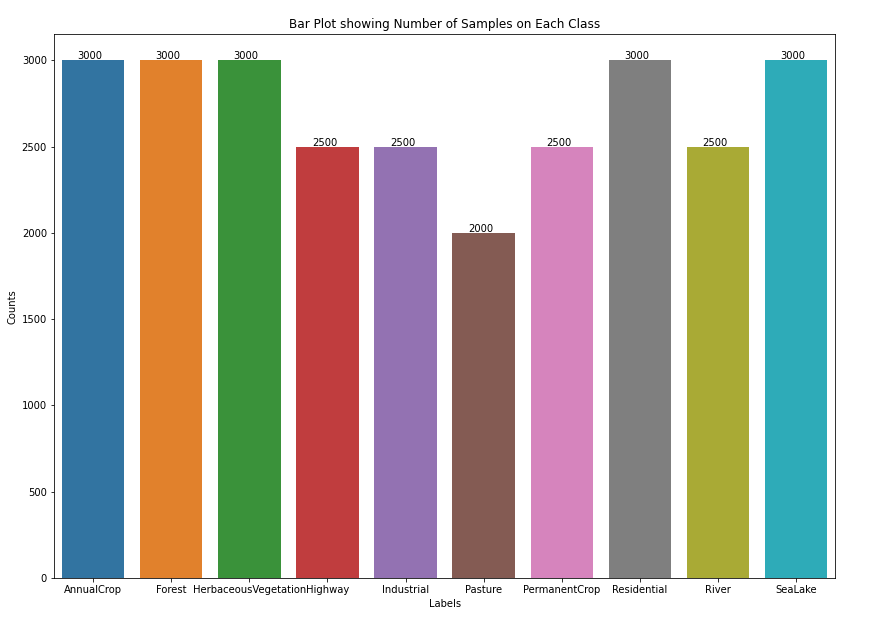
3,000 samples on half of the classes, others have 2,500 samples, while pasture only 2,000 samples.
Now let's take our training and validation sets and prepare them before training:
def prepare_for_training(ds, cache=True, batch_size=64, shuffle_buffer_size=1000):
  if cache:
    if isinstance(cache, str):
      ds = ds.cache(cache)
    else:
      ds = ds.cache()
  ds = ds.map(lambda d: (d["image"], tf.one_hot(d["label"], num_classes)))
  # shuffle the dataset
  ds = ds.shuffle(buffer_size=shuffle_buffer_size)
  # Repeat forever
  ds = ds.repeat()
  # split to batches
  ds = ds.batch(batch_size)
  # `prefetch` lets the dataset fetch batches in the background while the model
  # is training.
  ds = ds.prefetch(buffer_size=tf.data.experimental.AUTOTUNE)
  return ds
Here is what this function does:
cache(): This method saves the preprocessed dataset into a local cache file. This will only preprocess it the very first time (in the first epoch during training).map(): We map our dataset so each sample will be a tuple of an image and its corresponding label one-hot encoded withtf.one_hot().shuffle(): To shuffle the dataset so the samples are in random order.repeat()Every time we iterate over the dataset, it'll repeatedly generate samples for us; this will help us during the training.batch(): We batch our dataset into 64 or 32 samples per training step.prefetch(): This will enable us to fetch batches in the background while the model is training.
Let's run it for the training and validation sets:
batch_size = 64

# preprocess training & validation sets
train_ds = prepare_for_training(train_ds, batch_size=batch_size)
valid_ds = prepare_for_training(valid_ds, batch_size=batch_size)
Let's see what our data looks like:
# validating shapes
for el in valid_ds.take(1):
  print(el[0].shape, el[1].shape)
for el in train_ds.take(1):
  print(el[0].shape, el[1].shape)
Output:
(64, 64, 64, 3) (64, 10)
(64, 64, 64, 3) (64, 10)
Fantastic, both the training and validation have the same shape; where the batch size is 64, and the image shape is (64, 64, 3). The targets have the shape of (64, 10) as it's 64 samples with 10 classes one-hot encoded.
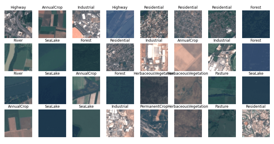
Let's visualize the first batch from the training dataset:
# take the first batch of the training set
batch = next(iter(train_ds))
def show_batch(batch):
plt.figure(figsize=(16, 16))
for n in range(min(32, batch_size)):
ax = plt.subplot(batch_size//8, 8, n + 1)
# show the image
plt.imshow(batch[0][n])
# and put the corresponding label as title upper to the image
plt.title(class_names[tf.argmax(batch[1][n].numpy())])
plt.axis('off')
plt.savefig("sample-images.png")
# showing a batch of images along with labels
show_batch(batch)Output:
Building the Model
Right. Now that we have our data prepared for training, let's build our model. First, downloading EfficientNetV2 and loading it as a hub.KerasLayer:
model_url = "https://tfhub.dev/google/imagenet/efficientnet_v2_imagenet1k_l/feature_vector/2"

# download & load the layer as a feature vector
keras_layer = hub.KerasLayer(model_url, output_shape=[1280], trainable=True)
We set the model_url to hub.KerasLayer so we get EfficientNetV2 as an image feature extractor. However, we set trainable to True so we're adjusting the pre-trained weights a bit for our dataset (i.e., fine-tuning).
Building the model:
m = tf.keras.Sequential([
  keras_layer,
  tf.keras.layers.Dense(num_classes, activation="softmax")
])
# build the model with input image shape as (64, 64, 3)
m.build([None, 64, 64, 3])
m.compile(
    loss="categorical_crossentropy",
    optimizer="adam",
    metrics=["accuracy", tfa.metrics.F1Score(num_classes)]
)m.summary()We use Sequential(), the first layer is the pre-trained CNN model, and we add a fully connected layer with the size of the number of classes as an output layer.
Finally, the model is built and compiled with categorical cross-entropy, adam optimizer, and accuracy and F1 score as metrics. Output:
Model: "sequential"
_________________________________________________________________
 Layer (type)                Output Shape              Param #
=================================================================
 keras_layer (KerasLayer)    (None, 1280)              117746848

 dense (Dense)               (None, 10)                12810

=================================================================
Total params: 117,759,658
Trainable params: 117,247,082
Non-trainable params: 512,576
_________________________________________________________________
Fine-tuning the Model
We have the data and model right, let's begin fine-tuning our model:
model_name = "satellite-classification"
model_path = os.path.join("results", model_name + ".h5")
model_checkpoint = tf.keras.callbacks.ModelCheckpoint(model_path, save_best_only=True, verbose=1)
# set the training & validation steps since we're using .repeat() on our dataset
# number of training steps
n_training_steps = int(num_examples * 0.6) // batch_size
# number of validation steps
n_validation_steps = int(num_examples * 0.2) // batch_size# train the model
history = m.fit(
train_ds, validation_data=valid_ds,
steps_per_epoch=n_training_steps,
validation_steps=n_validation_steps,
verbose=1, epochs=5,
callbacks=[model_checkpoint]
)The training will take several minutes, depending on your GPU. Here is the output:
Epoch 1/5
253/253 [==============================] - ETA: 0s - loss: 0.3780 - accuracy: 0.8859 - f1_score: 0.8832
Epoch 00001: val_loss improved from inf to 0.16415, saving model to results/satellite-classification.h5
253/253 [==============================] - 158s 438ms/step - loss: 0.3780 - accuracy: 0.8859 - f1_score: 0.8832 - val_loss: 0.1641 - val_accuracy: 0.9513 - val_f1_score: 0.9501
Epoch 2/5
253/253 [==============================] - ETA: 0s - loss: 0.1531 - accuracy: 0.9536 - f1_score: 0.9525
Epoch 00002: val_loss improved from 0.16415 to 0.12853, saving model to results/satellite-classification.h5
253/253 [==============================] - 106s 421ms/step - loss: 0.1531 - accuracy: 0.9536 - f1_score: 0.9525 - val_loss: 0.1285 - val_accuracy: 0.9568 - val_f1_score: 0.9559
Epoch 3/5
253/253 [==============================] - ETA: 0s - loss: 0.1092 - accuracy: 0.9660 - f1_score: 0.9654
Epoch 00003: val_loss improved from 0.12853 to 0.12095, saving model to results/satellite-classification.h5
253/253 [==============================] - 107s 424ms/step - loss: 0.1092 - accuracy: 0.9660 - f1_score: 0.9654 - val_loss: 0.1210 - val_accuracy: 0.9619 - val_f1_score: 0.9605
Epoch 4/5
253/253 [==============================] - ETA: 0s - loss: 0.1042 - accuracy: 0.9692 - f1_score: 0.9687
Epoch 00004: val_loss did not improve from 0.12095
253/253 [==============================] - 100s 394ms/step - loss: 0.1042 - accuracy: 0.9692 - f1_score: 0.9687 - val_loss: 0.1435 - val_accuracy: 0.9565 - val_f1_score: 0.9572
Epoch 5/5
253/253 [==============================] - ETA: 0s - loss: 0.1003 - accuracy: 0.9700 - f1_score: 0.9695
Epoch 00005: val_loss improved from 0.12095 to 0.09841, saving model to results/satellite-classification.h5
253/253 [==============================] - 107s 423ms/step - loss: 0.1003 - accuracy: 0.9700 - f1_score: 0.9695 - val_loss: 0.0984 - val_accuracy: 0.9702 - val_f1_score: 0.9687
As you can see, the model improved to about 97% accuracy on the validation set on epoch 5. You can increase the number of epochs to see whether it can improve further.
Model Evaluation
Up until now, we're only validating on the validation set during training. This section uses our model to predict satellite images that the model has never seen before. Loading the best weights:
# load the best weights
m.load_weights(model_path)
Extracting all the testing images and labels individually from test_ds:
# number of testing steps
n_testing_steps = int(all_ds[1].splits["train"].num_examples * 0.2)
# get all testing images as NumPy array
images = np.array([ d["image"] for d in test_ds.take(n_testing_steps) ])
print("images.shape:", images.shape)
# get all testing labels as NumPy array
labels = np.array([ d["label"] for d in test_ds.take(n_testing_steps) ])
print("labels.shape:", labels.shape)
Output:
images.shape: (5400, 64, 64, 3)
labels.shape: (5400,)
As expected, 5,400 images and labels, let's use the model to predict these images and then compare the predictions with the true labels:
# feed the images to get predictions
predictions = m.predict(images)
# perform argmax to get class index
predictions = np.argmax(predictions, axis=1)
print("predictions.shape:", predictions.shape)
Output:
predictions.shape: (5400,)from sklearn.metrics import f1_score
accuracy = tf.keras.metrics.Accuracy()
accuracy.update_state(labels, predictions)
print("Accuracy:", accuracy.result().numpy())
print("F1 Score:", f1_score(labels, predictions, average="macro"))Output:
Accuracy: 0.9677778
F1 Score: 0.9655686619720163
That's good accuracy! Let's draw the confusion matrix for all the classes:
# compute the confusion matrix
cmn = tf.math.confusion_matrix(labels, predictions).numpy()
# normalize the matrix to be in percentages
cmn = cmn.astype('float') / cmn.sum(axis=0)[:, np.newaxis]
# make a plot for the confusion matrix
fig, ax = plt.subplots(figsize=(10,10))
sns.heatmap(cmn, annot=True, fmt='.2f',
            xticklabels=[f"pred_{c}" for c in class_names],
            yticklabels=[f"true_{c}" for c in class_names],
            # cmap="Blues"
            cmap="rocket_r"
            )
plt.ylabel('Actual')
plt.xlabel('Predicted')
# plot the resulting confusion matrix
plt.savefig("confusion-matrix.png")
# plt.show()
Output:
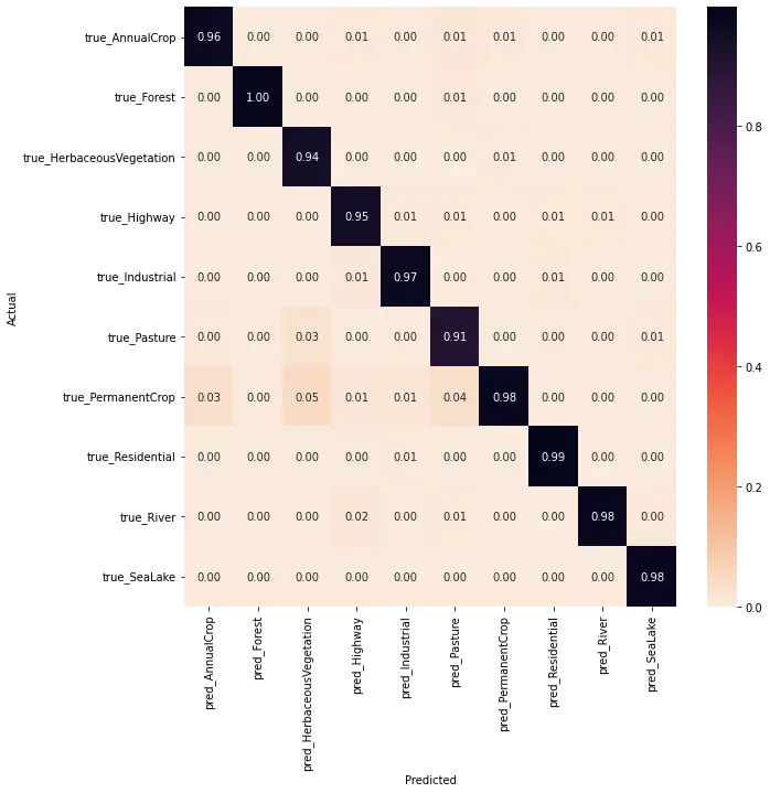 As you can see, the model is accurate in most of the classes, especially on forest images, as it achieved 100%. However, it's down to 91% for pasture, and the model sometimes predicts the pasture as permanent corp, also on herbaceous vegetation. Most of the confusion is between corp, pasture, and herbaceous vegetation as they all look similar and, most of the time, green from the satellite.
Let's show some examples that the model predicted:
def show_predicted_samples():
  plt.figure(figsize=(14, 14))
  for n in range(64):
      ax = plt.subplot(8, 8, n + 1)
      # show the image
      plt.imshow(images[n])
      # and put the corresponding label as title upper to the image
      if predictions[n] == labels[n]:
        # correct prediction
        ax.set_title(class_names[predictions[n]], color="green")
      else:
        # wrong prediction
        ax.set_title(f"{class_names[predictions[n]]}/T:{class_names[labels[n]]}", color="red")
      plt.axis('off')
      plt.savefig("predicted-sample-images.png")

# showing a batch of images along with predictions labels
show_predicted_samples()
Output:
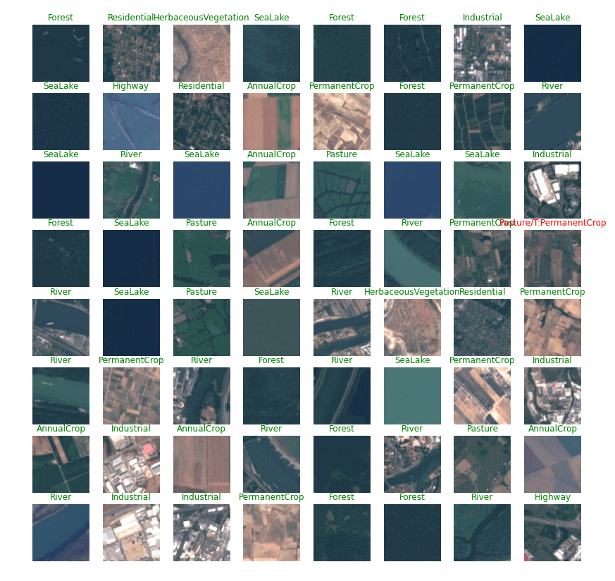 In all 64 images, only one (red label in the above image) failed to predict the actual class. It was predicted as a pasture where it should be a permanent crop.
Final Thoughts
Alright! That's it for the tutorial. If you want further improvement, I highly advise you to explore on TensorFlow hub, where you find the state-of-the-art pre-trained CNN models and feature extractors.
I also suggest you try out different optimizers and increase the number of epochs to see if you can improve it. You can use TensorBoard to track the accuracy of each change you make. Make sure you include the variables in the model name.
If you want more in-depth information, I encourage you to check the EuroSAT paper, where they achieved 98.57% accuracy with the 13 bands version of the dataset (1.93GB). You can also use this version of the dataset by passing "eurosat/all" instead of standard "eurosat" to the tfds.load() method.
You can get the complete code of this tutorial here.
Learn also: Skin Cancer Detection using TensorFlow in Python
Happy learning ♥
![]()
Why juggle between languages when you can convert? Check out our Code Converter. Try it out today!
View Full Code Understand My Code


Got a coding query or need some guidance before you comment? Check out this Python Code Assistant for expert advice and handy tips. It's like having a coding tutor right in your fingertips!