Juggling between coding languages? Let our Code Converter help. Your one-stop solution for language conversion. Start now!
In machine learning, and more specifically in classification (supervised learning), the industrial/raw datasets are known to get dealt with way more complications compared to toy data.
Among those constraints is the presence of a high imbalance ratio where usually, common classes happen way more frequently (majority) than the ones we actually target to study (minority).
In this tutorial, we will dive into more details on what lies underneath the Imbalance learning problem, how it impacts our models, understand what we mean by under/oversampling and implement using the Python library smote-variants.
Throughout the tutorial, we will use the fraudulent credit cards dataset from Kaggle, which you can download here.
Installation
$ pip install numpy pandas imblearn smote-variantsLearn also: Feature Selection using Scikit-Learn in Python
What is Imbalance Learning?
Imbalance Learning is in most cases present in the industry. As mentioned above, targeted classes (either for binary or multiclass problems) that need to be further studied and analyzed usually suffer from the lack of data in front of the tremendous presence of the common classes.
This imbalance holds a direct negative impact on the performance of the model while training, where it will get biased towards the majority class, and this may lead to falling under the accuracy paradox.
To better illustrate the accuracy paradox, imagine a dataset that contains 98 samples from class 0 and 2 from class 1, if our model predicts naively all of them as being 0 we will still have an accuracy of 98% which is relatively good even though our model just predicted by default all classes as 0. Such an accuracy value is misleading and can give wrong conclusions.
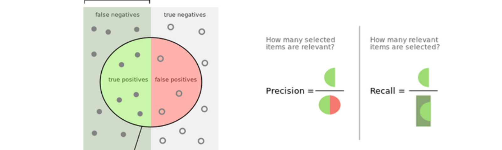
For this reason, we will now go through the used metrics when it comes to imbalanced datasets:
- Precision: Precision helps when the costs of false positives are high, so the bigger the precision the smaller the false positives rate.
- Recall: Recall helps when the costs of false negatives are high, so the bigger the recall the smaller the false negatives rate.
- F1-Score: it is the harmonic mean of precision and recall, in other words, it takes into consideration both of them, so the higher the f1 score the lower are the false negatives and false positive rates.
Another characteristic present in imbalance learning is known as the imbalance ratio. In the case of binary imbalanced classification, it is calculated by dividing the size of the minority class over the size of the majority one. We use the IR to know how severe the imbalance problem is.
Types Of Under/Oversampling
To reduce the imbalance ratio, we may pursue 2 different approaches, we can either reduce the majority classes (undersampling) or add samples to the minority ones (oversampling).
In this tutorial, we will go through 2 types of resampling-based approaches:
- Random sampling: Here we follow no given heuristic, we stochastically remove or duplicate the samples.
- Directed sampling: Unlike random sampling, here we follow a given heuristic/algorithm to choose the samples that need to be deleted in case of undersampling, or create and generate artificially data points for the minority ones when doing oversampling.
For the random sampling, we will use the imblearn Python library. But first, we will turn our CSV into a data frame format and store the labels into a variable y.
import numpy as np
import pandas as pd

df=pd.read_csv("creditcard.csv")

y=df["Class"]
X=df.drop(["Time","Class"],axis=1)
print(y.value_counts())
Output:
0    284315
1       492
Name: Class, dtype: int64
We will now create a RandomUnderSampler() object from imblearn and use the method fit_resample() to apply the undersampling on the dataset.
from imblearn.under_sampling import RandomUnderSampler

under=RandomUnderSampler()

X_und,y_und=under.fit_resample(X,y)

print(len(X_und[X_und==1])==len(X_und[X_und==0]))
Output:
TrueAs you can notice, after applying the undersampling the number of non-fraudulent credit cards is equal to the fraudulent ones.
For random oversampling, we use the same process, the only difference is to use RandomOverSampler() instead of RandomUnderSampler().
from imblearn.over_sampling import RandomOverSampler

over=RandomOverSampler()

X_und,y_und=over.fit_resample(X,y)

print(len(X_und[X_und==1])==len(X_und[X_und==0]))
Output:
TrueDirected Undersampling
Now we will dive into the second type of balancing algorithms which are the directed approaches.
For undersampling, we will cover those algorithms: Edited Nearest Neighbors, Instance Hardness Threshold, and TomekLinks.
- Edited Nearest Neighbors: in this undersampling technique, we remove majority samples where most of its neighbor is from the minority class.
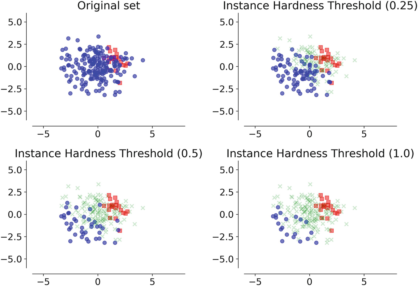
- Instance Hardness Threshold: Here we eliminate data points from the majority class that is being hard to classify. We basically use n classifiers and average the likelihood of misclassifying the instance, which is equal to 1 - Pi where Pi is the estimated probability prediction for sample i given a classifier.
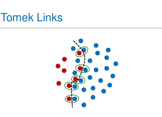
- TomekLinks: Here we delete the majority samples that have a tomeklink with a minority datapoint. A tomek link occurs when this formula is respected; given two samples x and y, for any other sample z we have: dist(x,y) < dist(x,z) and dist(x,y) < dist(y,z). In other words, minority and majority data points form a tomek link if they are the nearest neighbors to each other.
from imblearn.under_sampling import EditedNearestNeighbours,InstanceHardnessThreshold,TomekLinks

under_samp_models=[EditedNearestNeighbours(),InstanceHardnessThreshold,TomekLinks()]
for under_samp_model in under_samp_models:
    X_und,y_und=under_samp_model.fit_resample(X,y)
Directed Oversampling Using Smote
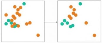
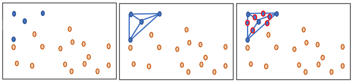
SMOTE ("Synthetic Minority Oversampling TEchnique") is an oversampling technique that works by drawing lines between the minority data points and generate data throughout those lines as shown in the figure below.
We will use the smote-variants Python library which is a package that includes 85 variants of smote, all mentioned by this scientific article.
The implementation is quite similar to the one of imblearn with minor changes like using the method sample() instead of fit_resample() to generate data. In this tutorial, we will use Kmeans_Smote, Safe_Level_Smote, and Smote_Cosine for the sake of examples.
import smote_variants as sv

svs=[sv.kmeans_SMOTE(),sv.Safe_Level_SMOTE(),sv.SMOTE_Cosine()]

for over_sampler in svs:
    X_over_samp, y_over_samp= over_sampler.sample(X, y)
Conclusion
Throughout this tutorial, we have learned:
- How to define an imbalance learning problem, and what is an imbalance ratio.
- Learn how to use the appropriate metrics to not fall into the accuracy paradox.
- Learn the difference between random and directed sampling.
- Use the Python libraries imblearn and smote-variants for undersampling and oversampling respectively.
Related: Detecting Fraudulent Transactions in a Streaming App using Kafka in Python
Happy learning ♥
Finished reading? Keep the learning going with our AI-powered Code Explainer. Try it now!
View Full Code Build My Python Code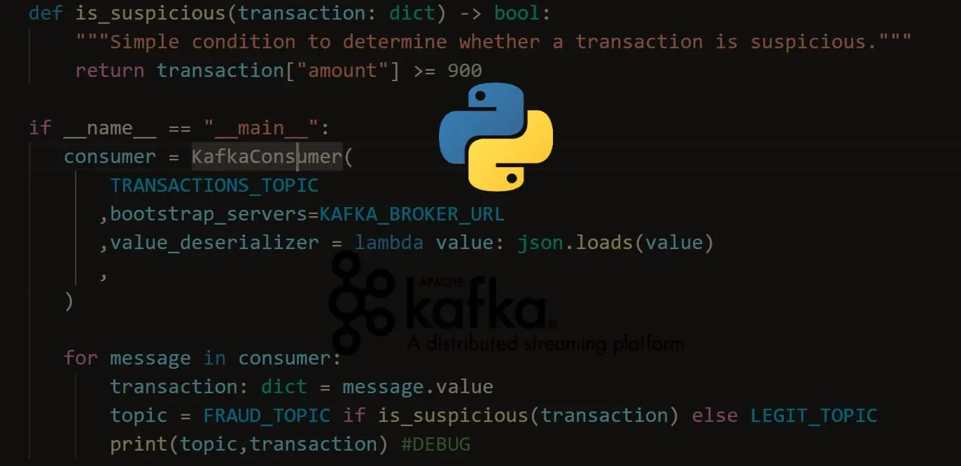


Got a coding query or need some guidance before you comment? Check out this Python Code Assistant for expert advice and handy tips. It's like having a coding tutor right in your fingertips!