How to Generate Images from Text using Stable Diffusion in Python

Kickstart your coding journey with our Python Code Assistant. An AI-powered assistant that's always ready to help. Don't miss out!

If you haven't been living under a rock, you have likely heard of the text-to-image AI models that can generate high-quality images from just text. Among the most well-known models in this field are DALLE-2 and GLIDE by OpenAI, Imagen by Google, Midjourney, Stable Diffusion, and many more.

All these text-to-image models come under the family of latent diffusion models. Hence, this in-depth tutorial will dive into the details of how latent diffusion models work and explore their inner workings. We will also write Python code to run a text-to-image model by dreamlike.art ourselves followed by manually implementing a diffusion framework. We will also see how to use the different components involved to generate similar images from a given image.

Table of content:

• Introduction
  • Prompt 1
  • Prompt 2
  • Prompt 3
• How do Latent Diffusion Models Work?
  • Guided Diffusion
    • Classifier Guidance
    • Classifier-free Guidance
• A Mathematical Perspective
  • Forward Diffusion
  • Backward Diffusion
  • Training to learn θ
• Code
  • Part 1: Using the Stable Diffusion Pipeline
  • Part 2: Manually Working with Different Components
    • Generating Similar Images for a Given Image
• Conclusion

Introduction

Latent diffusion models are a super popular family of models that can be used to create a wide variety of images, like drawings and paintings, portraits, landscapes, animals, the solar system, and basically anything you can imagine!

It can make several amazing images with prompts such as these:

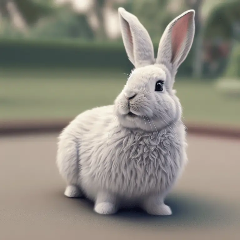
Prompt 1

“Cute Rabbit, Ultra HD, realistic, futuristic, sharp, octane render, photoshopped, photorealistic, soft, pastel, Aesthetic, Magical background”

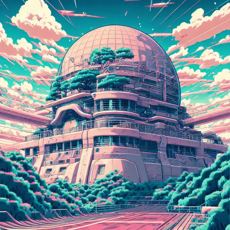
Prompt 2

“Anime style aesthetic landscape, 90's vintage style, digital art, ultra HD, 8k, photoshopped, sharp focus, surrealism, akira style, detailed line art”

Prompt 3

“Beautiful, abstract art of a human mind, 3D, highly detailed, 8K, aesthetic”

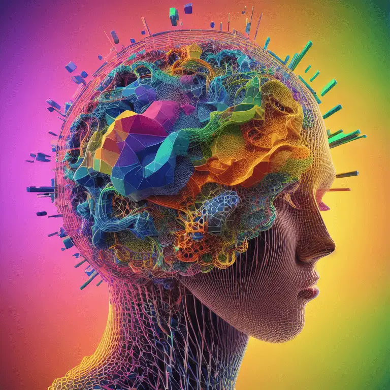
Who would have thought AI could generate images that are so beautiful and aesthetic!? It's hard to tell if an AI-generated the image of the rabbit or if it's a real photograph. Similarly, the anime-style landscape feels like an artwork by a professional artist! And the abstract art appears to have so many hidden meanings inside of it!

As we just saw, these generative models are really powerful. In fact, the more detailed a prompt is, the better and more relevant the image the model can make.

How do Latent Diffusion Models Work?

Let us now learn how these models generate images from nothing but text.

A latent diffusion model is a generative model that belongs to the family of Denoising Diffusion Probabilistic Models (DDPMs).

Simply put, the model works by decomposing the image generation process into a series of denoising steps. 

In essence, the process starts by generating some random noise and the model begins removing this noise during each denoising step, eventually resulting in an image.

To understand how the model learns to denoise the image, we need to learn the forward and backward diffusion processes.

The forward process aims to start with an image from our training set and turns it into pure noise. This is achieved by adding some noise at each step of the process for a set number of timesteps. While mathematically, it would take infinite steps to reach pure noise, adding noise for a few hundred steps provides a good approximation.

The backward process, also known as the reverse diffusion process or the generative model's sampling process, aims to recover the original image. It tries to teach a neural network that takes a noisy image as input and returns a slightly denoised image as its output. During each step of the process, the output of the forward process is given as input to the model, and the model tries to denoise this input, i.e., tries to predict the input of the forward process.

Note that the backward diffusion process is not the same as backpropagation.

Now that we have some idea about the diffusion model framework, let us get into a bit more depth and see the different components involved in the forward and backward process.

The Stable Diffusion framework consists of 4 components: an autoencoder, a text encoder and its tokenizer, a UNet model, and a scheduler:

1. The Variational Autoencoder is used to decode the images from the latent space into the pixel space. The latent space is a compressed representation of an image that captures the image's salient features. Since latent spaces are compressed (much lower dimensionality), it is computationally very much cheaper to work with the latent embeddings. The autoencoder is also used to encode the training images into embeddings for the model to learn while training.
   
2. The text encoder and its tokenizer help us get the user-specified text embeddings of the prompt for the image that needs to be generated. 
   
3. The U-Net model is what helps us denoise the latent image representations. A U-Net consists of a contracting and an expansive path, just like an autoencoder. However, a U-Net has skip connections, as shown in the image below. These skip connections help propagate information from the earlier layers alleviating the problem of vanishing gradients. Moreover, it helps retain the fine-grained details since we eventually lose information in the contractive path. The U-Nets used in the stable diffusion models consist of wide ResNet blocks and self-attention blocks, using techniques such as group normalization.
   
4. The scheduler is used to control the diffusion process. It maintains several things, such as the number of diffusion steps, how much noise is added on each step and the type of schedule to use (i.e., how to add noise, whether it always be constant or add more noise in the beginning and less in the end, etc.).

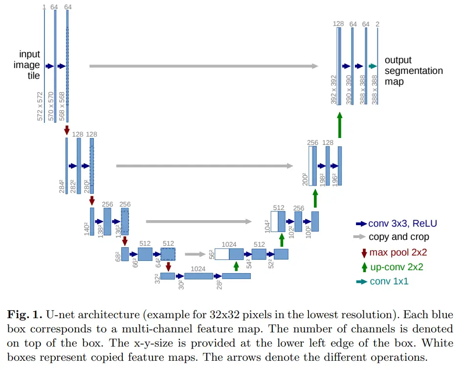The U-Net model architecture from the original paper.

Guided Diffusion

An essential aspect of these text-to-image models is conditioning on "something" to guide the diffusion process to favor the generation of specific images or classes. If there isn't any conditioning, there is no way for a model to know which image to generate, so it would generate any arbitrary random image.

There are mainly two families of methods for doing a guided diffusion.

Classifier Guidance

In this family of methods, we use another model, a classifier, trained on noisy images to predict the classes of its inputs. Using the gradients of this model, we can guide the diffusion process to our desired image! Check out this paper for more details.

Classifier-free Guidance

We can also achieve guidance without using a classifier model. In this family of models, we perform a single step of the diffusion process twice. Once conditioned on the text prompt and again without any conditioning. We get the noise predictions from both cases and use the following formula to get our overall noise term prediction:

ϵ=s∗ϵ(x|y)+(1−s)∗ϵ(x|0)
# or:
ϵ=ϵ(x|0)+s∗(ϵ(x|y)−ϵ(x|0)) # same equation as above

Here, ϵ(x|0) is unconditioned noise prediction, ϵ(x|y) is the conditioned noise prediction and ϵ is the final noise that we remove from our intermediate image.

Intuitively, the difference between the conditioned and the unconditioned noise terms gives us the direction for guidance. Suppose we scale this difference by s, our scaling factor. In that case, we are essentially going more towards the noise term, which, when removed, would lead to a conditioned image or, in other words, a guided reverse diffusion. Since this approach doesn't require a second model, it is used more often.

Finally, here's how our training pipeline looks like:

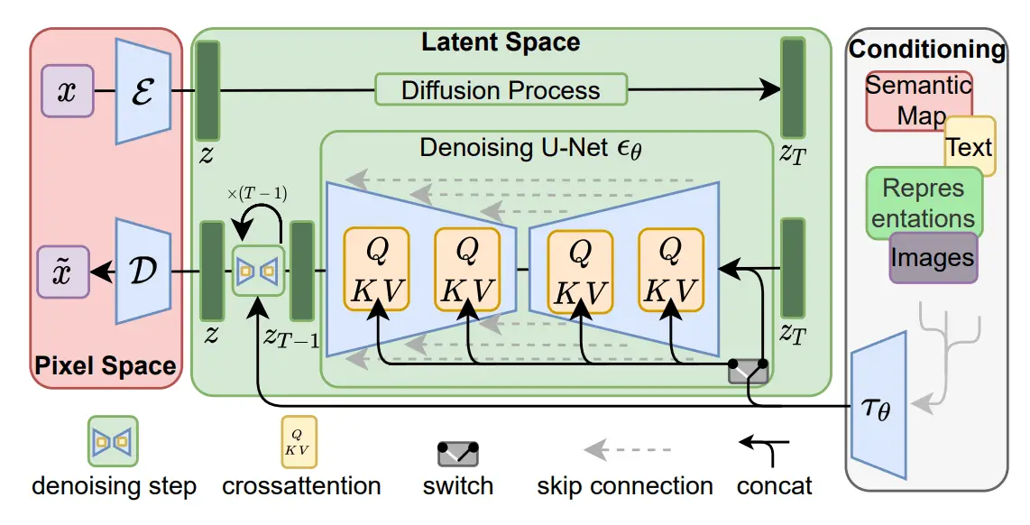The training pipeline in a nutshell from the Latent Diffusion Models paper 

During inference, we are only concerned with the denoising and so we ignore the diffusion process as shown in the image. Here are the steps for inference:

1. The user enters the text for the image to be generated. This text is the prompt of what the user wants the AI to generate as an image.
2. The text is converted into text embeddings by the tokenizer. Text embeddings are numerical representations of the input text that contain the semantic meaning of the sentence.
3. This embedding, along with some random noise vector, is sent to the U-Net. The random noise vector is an initial image representation in the form of latent variables, which will be refined through the U-Net to generate the final image.
4. The U-Net performs the backward diffusion process that iteratively updates the initial latent random noise vector to generate more meaningful and relevant image representations. The process is guided by the text embeddings and controlled by the scheduler using classifier or classifier-free guidance resulting in the latents for the final image. The scheduler assists in moving from the current sample to the previous one by subtracting the predicted noise, this process is repeated for a predefined number of inference steps (in our case we'll use 1000), with each step progressively updating the image latents to better match the input text description.
5. These final image latents are sent to the autoencoder for converting the latent space back into the pixel space, and we finally have our desired image.

Now that we have a pretty good idea about how diffusion models work, let's see how to generate our own images, like the ones at the beginning of this article!

Note: To get a more detailed insight into the diffusion process, check out the last section of this article, which discusses them from a mathematical perspective.

A Mathematical Perspective

Let's get a bit formal and define some notation.

T  = number of timesteps for the diffusion process

x₀   = Input image from the training set

q(x)  = Actual distribution of the training set

x_T   = Pure noise from which we would like to generate the original image

x_t   = intermediate latent space image at time step t

The entire diffusion process is formulated as a Markov Chain of T steps. A Markov chain is a stochastic model where we have a series of events with any event's probability distribution depending only on the immediate previous event. This means any denoising step in our backward diffusion depends only on the output of the previous timestep.

Forward Diffusion

The forward diffusion can be described as q(x_t|x_t-1)=N(x_t|1−β_t√x_t-1,β_tI)

This tells us at each step we are adding some Gaussian noise to x_t-1  to get the next noisy image x_t . The Gaussian noise we are adding has a mean 1-β_t√x_t-1  and variance β_tI . Here β_t is a hyperparameter that is generally controlled by the "Scheduler". It is also called the scale parameter and intuitively, controls the amount of pixel distribution. Hence a large beta would result in wider pixel distribution due to high variance and noise.

Backward Diffusion

The backward diffusion can be described as finding a probability distribution for q(x_t-1|x_t). Since this is intractable to compute, we choose a variational distribution p_θ  as a Gaussian distribution and parameterize it by the mean and the variance.  p_θ(x_t-1|x_t) = N(x_t-1|μ_θ(x_t,t),Σ_θ(x_t,t))

Repeatedly applying the above formula, we can get the distribution for the entire trajectory i.e. the entire reverse process.

p_θ(x_0:T) = p_θ(x_T) ∏ t=Tt=1 p_θ(x_t-1|x_t)

These parameters, θ, are exactly what's learned by the neural networks during the training. In practice, using a neural network as it is doesn't work too well and hence we use a U-Net instead.

Training to learn θ

Given our previous formulation, our goal now is to find the parameters θ that best approximate q. To do so, we formulate this by minimizing the KL-divergence between the two distributions which is equivalent to optimizing the Evidence Lower Bound aka ELBo.

If you have some experience with Bayesian models, this might seem quite familiar. If not, you can read more about variational inference (or variational autoencoders) in the popular book Pattern Recognition and Machine Learning by Christopher Bishop.

After lots of calculations (of which we would not go into the details), we get the loss function as follows:

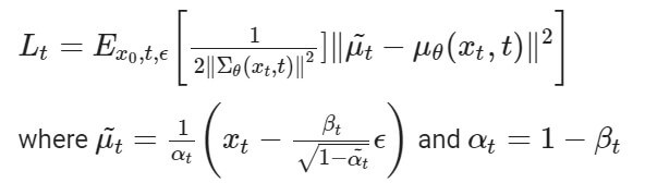
This is the loss that our neural network computes and does backpropagation to optimize the parameters! I invite you to check this blog post to learn more.

Related: How to Perform Image-to-Image Generation with Stable Diffusion in Python.

Code

Since stable diffusion models are open-sourced, you can run them yourself! Well, if you have decent computational resources at your hand you can try even bigger models since running these models is computationally expensive. You can check this link to see the inference benchmark on known GPUs.

Nevertheless, we are going to use only the GPUs provided to us by Google Colab and see how to generate images. Make sure you have GPU enabled. If not, go to Runtime then click on Change Runtime type, and from the hardware accelerator option select GPU.

Part 1: Using the Stable Diffusion Pipeline

We are first going to install the necessary libraries as follows:

%pip install --quiet --upgrade diffusers transformers accelerate

# The xformers package is mandatory to be able to create several 768x768 images & performance.
%pip install -q xformers==0.0.16rc425

Next we import the StableDiffusionPipeline and the PyTorch library.

from diffusers import StableDiffusionPipeline
import torch

Now we will be working using the dreamlike-art/dreamlike-photoreal-2.0 model that is hosted on the Huggingface hub, to generate images from our prompts. So we can load the entire pipeline in one go as follows:

model_id = "dreamlike-art/dreamlike-photoreal-2.0"
pipe = StableDiffusionPipeline.from_pretrained(model_id, torch_dtype=torch.float16)
pipe = pipe.to("cuda")

For the images above, we make a list of our prompts and a list of images that can store all the images generated:

prompts = ["Cute Rabbit, Ultra HD, realistic, futuristic, sharp, octane render, photoshopped, photorealistic, soft, pastel, Aesthetic, Magical background",
           "Anime style aesthetic landscape, 90's vintage style, digital art, ultra HD, 8k, photoshopped, sharp focus, surrealism, akira style, detailed line art",
           "Beautiful, abstract art of a human mind, 3D, highly detailed, 8K, aesthetic"]


images = []

Finally we can generate our images by passing the prompts one at a time to the instance of our Stable Diffusion pipeline.

for i, prompt in enumerate(prompts):
    image = pipe(prompt).images[0]
    image.save(f'result_{i}.jpg')
    images.append(image)

The generated images from these prompts are the same ones that were presented at the beginning of this article!

Part 2: Manually Working with Different Components

Let us write the code to manually use the four major components we discussed before to generate images.

Note: The code for working with the four components has been adapted from this Colab notebook.

We can now import all the libraries we need:

import torch
from torch import autocast
import numpy as np

from transformers import CLIPTextModel, CLIPTokenizer

from diffusers import AutoencoderKL
from diffusers import LMSDiscreteScheduler
from diffusers import UNet2DConditionModel
from diffusers.schedulers.scheduling_ddim import DDIMScheduler

from tqdm import tqdm
from PIL import Image

Let us define a Python class for the diffusion model we will code ourselves:

class ImageDiffusionModel:

    def __init__(self, vae, tokenizer, text_encoder, unet, 
                 scheduler_LMS, scheduler_DDIM):
        self.vae = vae
        self.tokenizer = tokenizer
        self.text_encoder = text_encoder
        self.unet = unet
        self.scheduler_LMS = scheduler_LMS
        self.scheduler_DDIM = scheduler_DDIM
        self.device = 'cuda' if torch.cuda.is_available() else 'cpu'

Here we have defined 2 schedulers. We will be working with the DDIM scheduler later on.

Now we need several helper methods to generate an image. In the pipeline we discussed above, we first need to convert text from the prompt by the user into text embeddings:

    def get_text_embeds(self, text):
        # tokenize the text
        text_input = self.tokenizer(text, 
                                    padding='max_length', 
                                    max_length=tokenizer.model_max_length, 
                                    truncation=True, 
                                    return_tensors='pt')
        # embed the text
        with torch.no_grad():
            text_embeds = self.text_encoder(text_input.input_ids.to(self.device))[0]
        return text_embeds

    def get_prompt_embeds(self, prompt):
        # get conditional prompt embeddings
        cond_embeds = self.get_text_embeds(prompt)
        # get unconditional prompt embeddings
        uncond_embeds = self.get_text_embeds([''] * len(prompt))
        # concatenate the above 2 embeds
        prompt_embeds = torch.cat([uncond_embeds, cond_embeds])
        return prompt_embeds

Here we have first defined a helper method to return text embeddings as PyTorch tensors for a given text. We will be doing classifier-free guidance to get the embeddings for the user's prompt. Hence we first generate text embeddings for both the prompt and an empty string and then concatenate them. 

Now our diffusion model class needs a method to generate the latent image embeddings after doing the reverse diffusion process, which, when decoded, gives us the actual image:

    def get_img_latents(self, 
                        text_embeds, 
                        height=512, width=512, 
                        num_inference_steps=50, 
                        guidance_scale=7.5, 
                        img_latents=None):
        # if no image latent is passed, start reverse diffusion with random noise
        if img_latents is None:
            img_latents = torch.randn((text_embeds.shape[0] // 2, self.unet.in_channels,\
                                       height // 8, width // 8)).to(self.device)
        # set the number of inference steps for the scheduler
        self.scheduler_LMS.set_timesteps(num_inference_steps)
        # scale the latent embeds
        img_latents = img_latents * self.scheduler_LMS.sigmas[0]
        # use autocast for automatic mixed precision (AMP) inference
        with autocast('cuda'):
            for i, t in tqdm(enumerate(self.scheduler_LMS.timesteps)):
                # do a single forward pass for both the conditional and unconditional latents
                latent_model_input = torch.cat([img_latents] * 2)
                sigma = self.scheduler_LMS.sigmas[i]
                latent_model_input = latent_model_input / ((sigma ** 2 + 1) ** 0.5)
                # predict noise residuals
                with torch.no_grad():
                    noise_pred = self.unet(latent_model_input, t, encoder_hidden_states=text_embeds)['sample']
                # separate predictions for unconditional and conditional outputs
                noise_pred_uncond, noise_pred_cond = noise_pred.chunk(2)
                # perform guidance
                noise_pred = noise_pred_uncond + guidance_scale * (noise_pred_cond - noise_pred_uncond)
                # remove the noise from the current sample i.e. go from x_t to x_{t-1}
                img_latents = self.scheduler_LMS.step(noise_pred, i, img_latents)['prev_sample']
        return img_latents

In the method above:

• We first check if the user has sent some image embeddings. If not, we generate random latents of the appropriate shape. Notice that the shape's first dimension is set as the first dimension of the text embeddings divided by two. This is because we have two text embeddings for each prompt as we are performing classifier-free guidance.
• We then set the number of inference steps and scale the latent embeddings.
• Next, we use the automatic mixed precision (AMP) inference context manager to do the reverse diffusion process. AMP is a PyTorch feature allowing us to use lower-precision arithmetic (like float16 instead of float64 or float32) for certain model parts without sacrificing accuracy.
• For each step in the reverse diffusion, we want to do a forward pass on both the conditional and unconditional text embeddings, so we replicate the latent image embeddings twice, scale them using sigma for the i-th step and predict the noise residuals.
• We separate the noise residuals for conditional and unconditional texts and use those to calculate the noise predictions using guidance. This is the final noise we get, which is then removed from the image using the step method of the scheduler.

Now we need a method to decode the image from the latent space into the pixel space and transform this into a suitable PIL image format:

    def decode_img_latents(self, img_latents):
        img_latents = img_latents / 0.18215
        with torch.no_grad():
            imgs = self.vae.decode(img_latents)
        # load image in the CPU
        imgs = imgs.detach().cpu()
        return imgs

    def transform_imgs(self, imgs):
        # transform images from the range [-1, 1] to [0, 1]
        imgs = (imgs / 2 + 0.5).clamp(0, 1)
        # permute the channels and convert to numpy arrays
        imgs = imgs.permute(0, 2, 3, 1).numpy()
        # scale images to the range [0, 255] and convert to int
        imgs = (imgs * 255).round().astype('uint8')        
        # convert to PIL Image objects
        imgs = [Image.fromarray(img) for img in imgs]
        return imgs

In the decode_img_latents() method, we have first divided the image embeddings by 0.18215 since the authors also proposed this in their paper. We then use a Variational Autoencoder (VAE) to decode the latent embeddings.

Next, the transform_imgs() method takes the image we received from the previous function and scales it appropriately so that the pixels range from 0 to 255 instead of -1 to 1. The color channels are also swapped, and pixels are rounded to integers to represent the images in the PIL image format.

We now have all the pieces, we're ready to code our prompt_to_img() method:

    def prompt_to_img(self, 
                      prompts, 
                      height=512, width=512, 
                      num_inference_steps=50, 
                      guidance_scale=7.5, 
                      img_latents=None):
        # convert prompt to a list
        if isinstance(prompts, str):
            prompts = [prompts]
        # get prompt embeddings
        text_embeds = self.get_prompt_embeds(prompts)
        # get image embeddings
        img_latents = self.get_img_latents(text_embeds,
                                      height, width,
                                      num_inference_steps,
                                      guidance_scale, 
                                      img_latents)
        # decode the image embeddings
        imgs = self.decode_img_latents(img_latents)
        # convert decoded image to suitable PIL Image format
        imgs = self.transform_imgs(imgs)
        return imgs

In this code, we first convert the prompt by the user to a list, convert this list to get the text embeddings, perform the reverse diffusion process using these embeddings, decode the latent image embeddings, and finally transform the decoded output for the PIL image format. That's all there is to code to generate images ourselves!

Before generating images, let us load the necessary pre-trained components from the Huggingface Transformers and the diffusers library:

device = 'cuda'
# Load autoencoder
vae = AutoencoderKL.from_pretrained('CompVis/stable-diffusion-v1-4', 
                                    subfolder='vae').to(device)
# Load tokenizer and the text encoder
tokenizer = CLIPTokenizer.from_pretrained('openai/clip-vit-large-patch14')
text_encoder = CLIPTextModel.from_pretrained('openai/clip-vit-large-patch14').to(device)
# Load UNet model
unet = UNet2DConditionModel.from_pretrained('CompVis/stable-diffusion-v1-4', subfolder='unet').to(device)
# Load schedulers
scheduler_LMS = LMSDiscreteScheduler(beta_start=0.00085, 
                                 beta_end=0.012, 
                                 beta_schedule='scaled_linear', 
                                 num_train_timesteps=1000)

scheduler_DDIM = DDIMScheduler(beta_start=0.00085, 
                               beta_end=0.012, 
                               beta_schedule='scaled_linear', 
                               num_train_timesteps=1000)

Let us now create an instance of the defined class and generate some images:

model = ImageDiffusionModel(vae, tokenizer, text_encoder, unet, scheduler_LMS, scheduler_DDIM)

prompts = ["A really giant cute pink barbie doll on the top of Burj Khalifa", 
           "A green, scary aesthetic dragon breathing fire near a group of heroic firefighters"]

imgs = model.prompt_to_img(prompts)

imgs[0]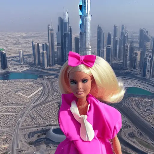

imgs[1]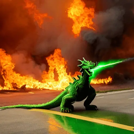

Here we pass a single text prompt to the instance of ImageDiffusionModel to get the following generated image.

We can generate any image this way. You can try out more examples yourself!

Let us generate images with the same prompts we used in the StableDiffusionPipeline:

prompts = ["Cute Rabbit, Ultra HD, realistic, futuristic, sharp, octane render, photoshopped, photorealistic, soft, pastel, Aesthetic, Magical background",
           "Anime style aesthetic landscape, 90's vintage style, digital art, ultra HD, 8k, photoshopped, sharp focus, surrealism, akira style, detailed line art",
           "Beautiful, abstract art of a human mind, 3D, highly detailed, 8K, aesthetic"]

imgs = model.prompt_to_img(prompts)

imgs[0]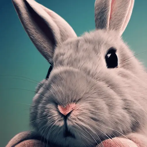

These outputs are so much different than the ones we got before. The model “dreamlike-art/dreamlike-photoreal-2.0” is definitely much better at producing more aesthetically pleasing images.

The framework we just implemented is incredibly powerful. Just by modifying a few parts and putting things here and there, we can do a lot of amazing things, such as generating videos, image inpainting, getting similar images, and much more. In this tutorial, we will only explore how to get more similar images for an image.

Generating Similar Images for a Given Image

Please note that we have a separate tutorial on how to do that using depth estimation, check it out here.

Once you understand how to generate an individual image, creating similar images for a given image is quite easy. To do this, we need to convert our original image into the latent embedding space, add some noise and do the reverse diffusion process starting somewhere between. We start somewhere in between because our noisy image embedding would provide a good reference for the reverse diffusion process.

To do all this, we will use the DDIM scheduler, which is more suited for image-to-image tasks. The LMSDiscrete scheduler doesn't work too well when the reverse diffusion process begins from an intermediate timestep. Let us now add a slightly modified version of the get_img_latents() method that adapts for this particular scheduler:

    def get_img_latents_similar(self,
                                img_latents,
                                text_embeds, 
                                height=512, width=512, 
                                num_inference_steps=50, 
                                guidance_scale=7.5,
                                start_step=10):
        # set the number of inference steps for the scheduler
        self.scheduler_DDIM.set_timesteps(num_inference_steps)
        if start_step > 0:
            start_timestep = self.scheduler_DDIM.timesteps[start_step]
            start_timesteps = start_timestep.repeat(img_latents.shape[0]).long()
            # add noise to the image latents
            noise = torch.randn_like(img_latents)
            img_latents = self.scheduler_DDIM.add_noise(img_latents, noise, start_timesteps)
        # use autocast for automatic mixed precision (AMP) inference
        with autocast('cuda'):
            for i, t in tqdm(enumerate(self.scheduler_DDIM.timesteps[start_step:])):
                # do a single forward pass for both the conditional and unconditional latents
                latent_model_input = torch.cat([img_latents] * 2)
                # predict noise residuals
                with torch.no_grad():
                    noise_pred = self.unet(latent_model_input, t, encoder_hidden_states=text_embeds)['sample']
                # separate predictions for unconditional and conditional outputs
                noise_pred_uncond, noise_pred_cond = noise_pred.chunk(2)
                # perform guidance
                noise_pred = noise_pred_uncond + guidance_scale * (noise_pred_cond - noise_pred_uncond)
                # remove the noise from the current sample i.e. go from x_t to x_{t-1}
                img_latents = self.scheduler_DDIM.step(noise_pred, t, img_latents)['prev_sample']
        return img_latents

We have a few important distinctions to make here. First, in this method, img_latents is no longer a default argument. We have also included another argument, start_step, to specify the timestep from which to begin the reverse diffusion process. Also, notice how we add noise to the image embeddings using the DDIM scheduler and don't scale the image embeddings anymore.

Next, we define the following method to generate similar images:

    def similar_imgs(self, 
                     img, 
                     prompt, 
                     height=512, width=512,
                     num_inference_steps=50, 
                     guidance_scale=7.5,
                     start_step=10):
        # get image latents
        img_latents = self.encode_img_latents(img)
        if isinstance(prompt, str):
            prompt = [prompt]
        # get prompt embeddings
        text_embeds = self.get_prompt_embeds(prompt)
        img_latents = self.get_img_latents_similar(img_latents=img_latents,
                                                   text_embeds=text_embeds,
                                                height=height, width=width,
                                                num_inference_steps=num_inference_steps,
                                                guidance_scale=guidance_scale,
                                                start_step=start_step) 
        # decode the image embeddings
        imgs = self.decode_img_latents(img_latents)
        # convert decoded image to suitable PIL Image format
        imgs = self.transform_imgs(imgs)
        return imgs

We first encode the image from the pixel to the latent embedding space. The prompt text is converted into a Python list from which we get the prompt text embeddings using the methods we previously defined. We pass these embeddings to the get_img_latents_similar() method. Then we decode the final image latents that we get and transform it to the format suitable for the PIL library.

Now to test our new functionality, let’s generate an image using our model and then generate more similar images to this image.

model = ImageDiffusionModel(vae, tokenizer, text_encoder, unet, scheduler_LMS, scheduler_DDIM)
prompt = ["Aesthetic star wars spaceship with an aethethic background, Ultra HD, futuristic, sharp, octane render, neon"]
imgs = model.prompt_to_img(prompt)
imgs[0]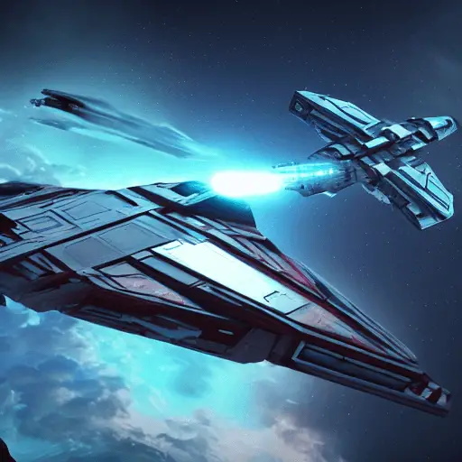

We can save this image to our computer and load it as follows. We do this extra step to demonstrate one could also have loaded their own image:

# saving the image
imgs[0].save("spaceship1.png")
# load it
original_img = Image.open("spaceship1.png")
original_img

prompt = "Aesthetic star wars spaceship"
# generate similar images to the original image guided with the prompt
imgs = model.similar_imgs(original_img, prompt,
                          num_inference_steps=20,
                          start_step=7)
imgs[0]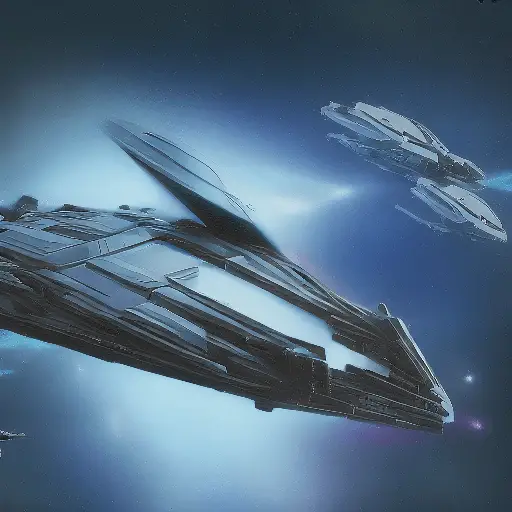

They look quite similar, don't they? Let us try changing the prompt a little bit.

prompt = "Aesthetic star wars spaceship with a scary background"
imgs = model.similar_imgs(original_img, prompt,
                          num_inference_steps=20,
                          start_step=7)
imgs[0]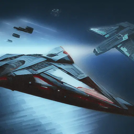

Hurray, another similar image! Note that we can control how similar the images look by appropriately choosing the number of inference steps and the starting step. We can of course also change the prompts to vary the image.

Conclusion

This was fun! In this article, we learned about how stable diffusion (and other latent diffusion models) work in quite a lot of depth. We also saw how to generate images ourselves from prompts using a model loaded from Hugging Face. We then saw how to work with the different components involved and also learned how to generate similar images from a given image. Now go ahead and create beautiful aesthetic images!

Learn also: Image Captioning using PyTorch and Transformers in Python.

Happy generating ♥

References

• https://huggingface.co/dreamlike-art/dreamlike-photoreal-2.0
• https://huggingface.co/CompVis/stable-diffusion-v1-4
• How diffusion models work: the math from scratch
• Stable Diffusion - What, Why, How? - YouTube

Save time and energy with our Python Code Generator. Why start from scratch when you can generate? Give it a try!

Read Also

How to Fine Tune ViT for Image Classification using Transformers in Python

Learn how to fine tune the Vision Transformer (ViT) model for the image classification task using the Huggingface Transformers, evaluate, and datasets libraries in Python.

Image Captioning using PyTorch and Transformers in Python

Learn how to use pre-trained image captioning transformer models and what are the metrics used to compare models, you'll also learn how to train your own image captioning model with Pytorch and transformers in Python.

Image to Image Generation with Stable Diffusion in Python

Learn how you can generate similar images with depth estimation (depth2img) using stable diffusion with huggingface diffusers and transformers libraries in Python.

Comment panel