How to Generate and Visualize Text Embeddings in Python

Want to code faster? Our Python Code Generator lets you create Python scripts with just a few clicks. Try it now!

Take two sentences:

"The dog played in the park."
"A canine ran through the green field."

Not a single word overlaps. Not one. A keyword search would rate these as completely unrelated. But any human — and any decent language model — immediately recognizes they describe the same thing. The meaning matches, even though the vocabulary doesn't.

This ability to capture meaning independent of word choice is what makes text embeddings one of the most important concepts in modern AI. Embeddings are the foundation of semantic search, recommendation systems, chatbots, and retrieval-augmented generation. Yet most developers treat them as a black box — feed text in, get numbers out, hope for the best.

In this tutorial, I'll crack that box open. We'll generate embeddings for 50 sentences across 10 categories, compare their semantic similarities, and produce four detailed visualizations — PCA, t-SNE, cosine similarity heatmaps, and dimension analysis — that reveal exactly what embeddings capture and how they work.

What Text Embeddings Actually Are

An embedding is a list of numbers that represents what a piece of text means. Not what it says — what it means. The sentence "The dog played in the park" might become a vector like:

[-0.06, 0.05, -0.02, 0.00, -0.01, -0.16, -0.03, -0.02, ...]

Each number is a coordinate in a 384-dimensional space (or 768, or 1536 — depends on the model). Sentences with similar meanings end up near each other in this space. "A canine ran through the green field" will be close to "The dog played in the park," while "The stock market crashed yesterday" will be far away.

The model that produces these embeddings — in our case, a sentence transformer — was trained on billions of sentence pairs. It learned which sentences are paraphrases of each other and which aren't. That training compressed an enormous amount of linguistic knowledge into those 384 numbers. For more background on how transformer models learn these representations, check out our guide to fine-tuning BERT for text classification, which covers the architecture that makes embeddings possible.

Setup: One pip install

pip install sentence-transformers numpy matplotlib seaborn scikit-learn

That's it. No API keys, no GPU, no Docker. Sentence Transformers runs on CPU and produces quality embeddings in milliseconds per sentence.

Step 1: Build a Diverse Sentence Corpus

To understand embeddings, we need sentences that span different topics. I created 50 sentences across 10 categories — Technology, Animals, Food, Travel, Emotions, Science, Sports, Art, Business, and Health. Five sentences per category. Here's a sample:

sentences = [
    # Technology
    "The computer processed data at incredible speed",
    "Machine learning models require large amounts of training data",
    "Python is widely used for artificial intelligence applications",

    # Animals
    "The dog chased the ball across the green field",
    "Cats are independent creatures that enjoy solitude",
    "The majestic eagle soared high above the mountains",

    # Food
    "The chef prepared a delicious Italian pasta dish",
    "Fresh ingredients make the best homemade meals",
    "The chocolate cake was rich and decadently sweet",

    # ... 50 sentences, 10 categories
]

This diversity is critical — it means we'll see distinct clusters in our visualizations, which reveals whether the model is actually capturing semantic categories or just grouping by superficial word overlap.

Step 2: Generate Embeddings

One function call converts all 50 sentences into vectors:

from sentence_transformers import SentenceTransformer
import numpy as np

model = SentenceTransformer("all-MiniLM-L6-v2")
embeddings = model.encode(
    sentences,
    convert_to_numpy=True,
    normalize_embeddings=True,  # L2 normalization
)

print(embeddings.shape)  # (50, 384)
print(embeddings[0][:8])  # First 8 values of first sentence
# [-0.0599  0.054  -0.0241  0.0022 -0.0091 -0.1615 -0.0259 -0.0178]

Fifty sentences became fifty vectors of 384 numbers each. The model loaded in about 2 seconds (first run downloads 80MB; subsequent runs use cache), and encoding all 50 sentences took under a second.

Why 384 dimensions? The all-MiniLM-L6-v2 model is a distilled version of a larger model — it compresses linguistic knowledge into a compact 384-dim vector. Production models like all-mpnet-base-v2 use 768 dimensions for higher quality at the cost of 2-3x slower inference. Start with MiniLM for prototyping, upgrade to mpnet for production.

Step 3: Visualize with PCA

You can't visualize 384 dimensions directly, but PCA (Principal Component Analysis) projects them down to 2D while preserving as much structure as possible:

from sklearn.decomposition import PCA
import matplotlib.pyplot as plt

pca = PCA(n_components=2, random_state=42)
embeddings_2d = pca.fit_transform(embeddings)

# Color each category differently
categories = ["Tech", "Animals", "Food", "Travel", "Emotions", 
              "Science", "Sports", "Art", "Business", "Health"]
colors = ["#3b82f6", "#10b981", "#f59e0b", "#8b5cf6", "#ef4444",
          "#06b6d4", "#f97316", "#ec4899", "#6366f1", "#14b8a6"]

fig, ax = plt.subplots(figsize=(16, 11))
for cat, color in zip(categories, colors):
    mask = [c == cat for c in categories_by_sentence]
    ax.scatter(embeddings_2d[mask, 0], embeddings_2d[mask, 1],
               c=color, label=cat, alpha=0.75, s=120, edgecolors='white')

ax.set_title("Text Embeddings Visualized with PCA\n"
             "50 sentences → 384-dim vectors → 2D projection")
ax.legend()
plt.savefig("pca_visualization.png", dpi=180)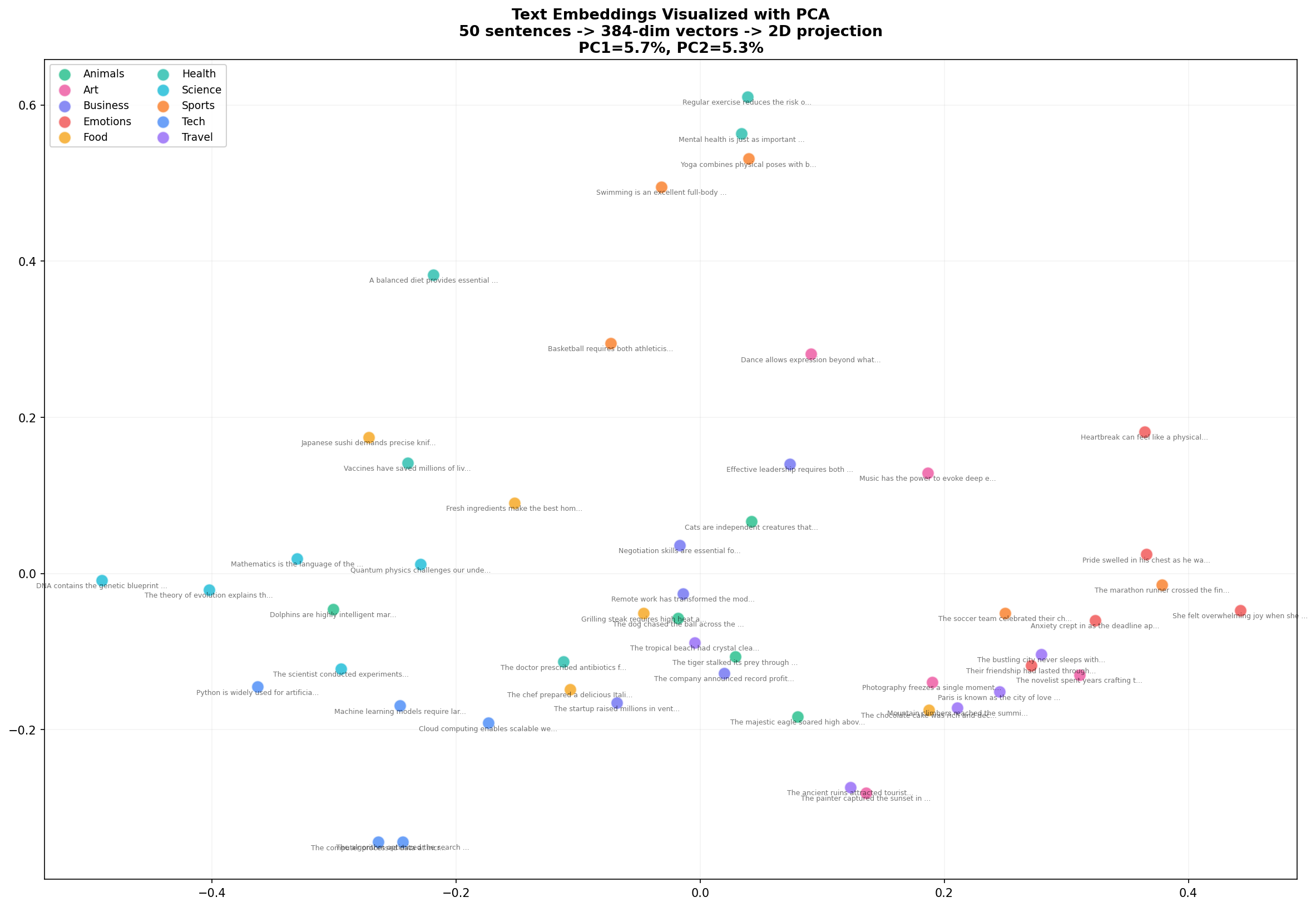

Look at what emerges. Food sentences (yellow) cluster together on the left. Animals (green) form a group in the upper region. Tech and Business (blue, indigo) mix in the lower right — which makes sense, since many tech sentences involve business concepts. PC1 and PC2 together explain about 10% of the variance, which is impressive considering we compressed 384 dimensions into 2.

Step 4: Visualize with t-SNE

PCA is fast but limited — it can only capture linear relationships. t-SNE is slower but reveals much richer structure by preserving local neighborhoods:

from sklearn.manifold import TSNE

tsne = TSNE(n_components=2, perplexity=8, random_state=42, max_iter=1000)
embeddings_2d_tsne = tsne.fit_transform(embeddings)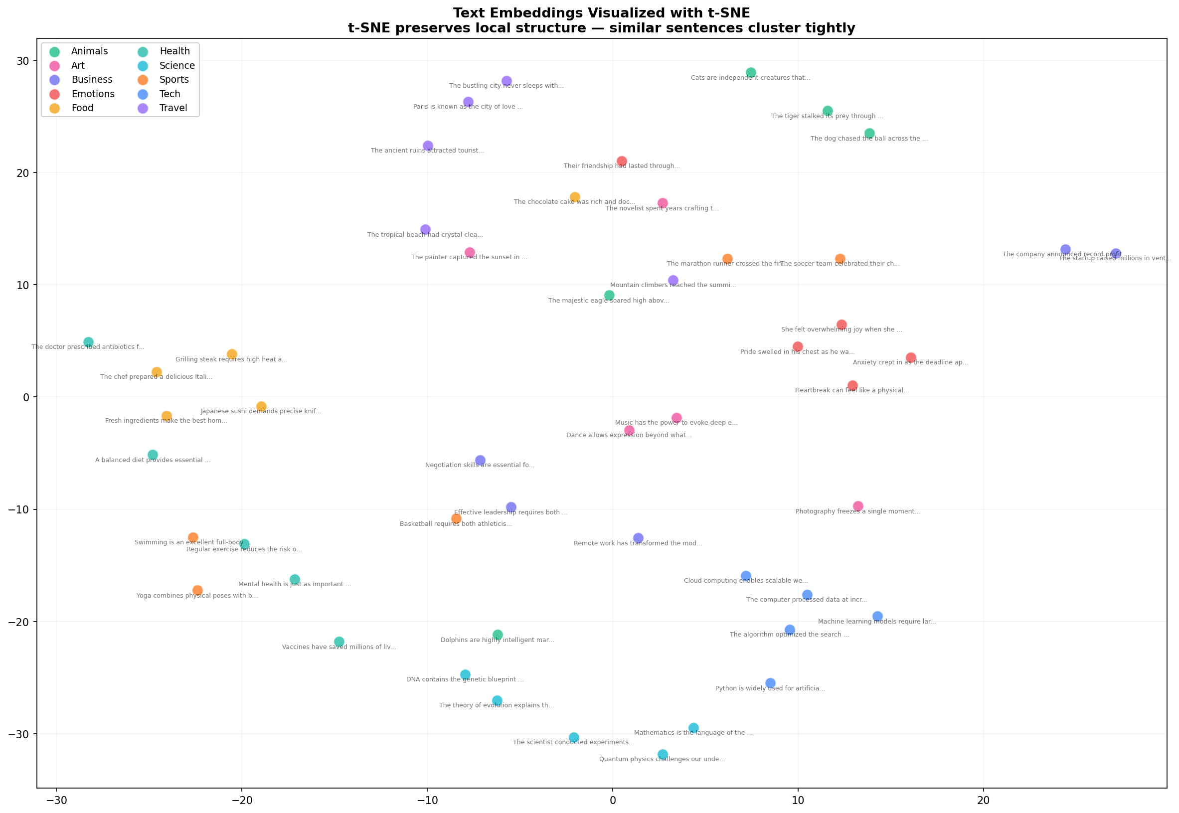

t-SNE reveals what PCA couldn't: tight, well-separated clusters. Health sentences (teal) now form a distinct group. Art sentences (pink) cluster together. The Business and Tech sentences that mixed in PCA are now more clearly separated. This is why t-SNE is the go-to for embedding visualization — it preserves the local structure that matters for semantic similarity.

The trade-off: t-SNE is stochastic (different runs produce different layouts) and its axes have no interpretable meaning unlike PCA. Use PCA for quick exploration, t-SNE for publication-quality figures.

Step 5: Cosine Similarity Heatmap

Scatter plots show clusters, but they don't show pairwise similarity. For that, we need a heatmap:

from sklearn.metrics.pairwise import cosine_similarity
import seaborn as sns

# Select one sentence per category for readability
indices = [0, 5, 10, 15, 20, 25, 30, 35, 40, 45]
subset = embeddings[indices]

sim_matrix = cosine_similarity(subset)

fig, ax = plt.subplots(figsize=(14, 12))
sns.heatmap(sim_matrix, annot=True, fmt=".2f", cmap="YlOrRd",
            xticklabels=labels, yticklabels=labels,
            vmin=0, vmax=1, ax=ax)
ax.set_title("Cosine Similarity Between Sentence Embeddings\n"
             "1.0 = identical meaning, 0.0 = completely unrelated")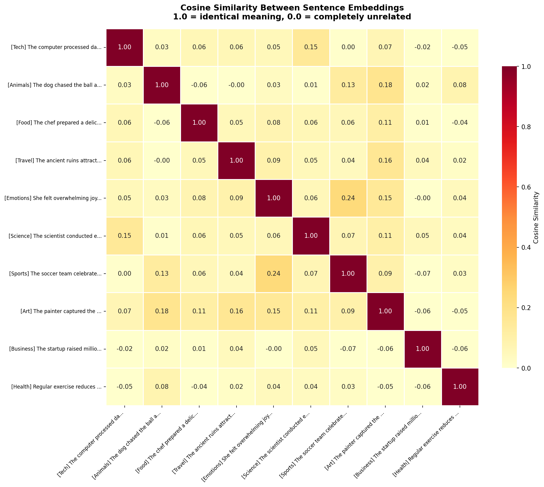

The diagonal is 1.0 — every sentence is perfectly similar to itself. But look at the off-diagonal cells. The Tech sentence (row 1) has 0.36 similarity with Business, 0.19 with Science — moderate, reasonable relationships. Against Food (0.09) and Animals (0.14), the similarity drops near zero. The model correctly identifies which topics are related and which aren't.

The heatmap also reveals nuanced relationships. Emotions and Art have a 0.16 similarity — not huge, but notably higher than Emotions vs Sports (0.08). The model has learned that emotional expression and artistic expression share conceptual ground.

Step 6: Dimension Distribution Analysis

Those 384 numbers — are they all equally important? Let's analyze how information is distributed across dimensions:

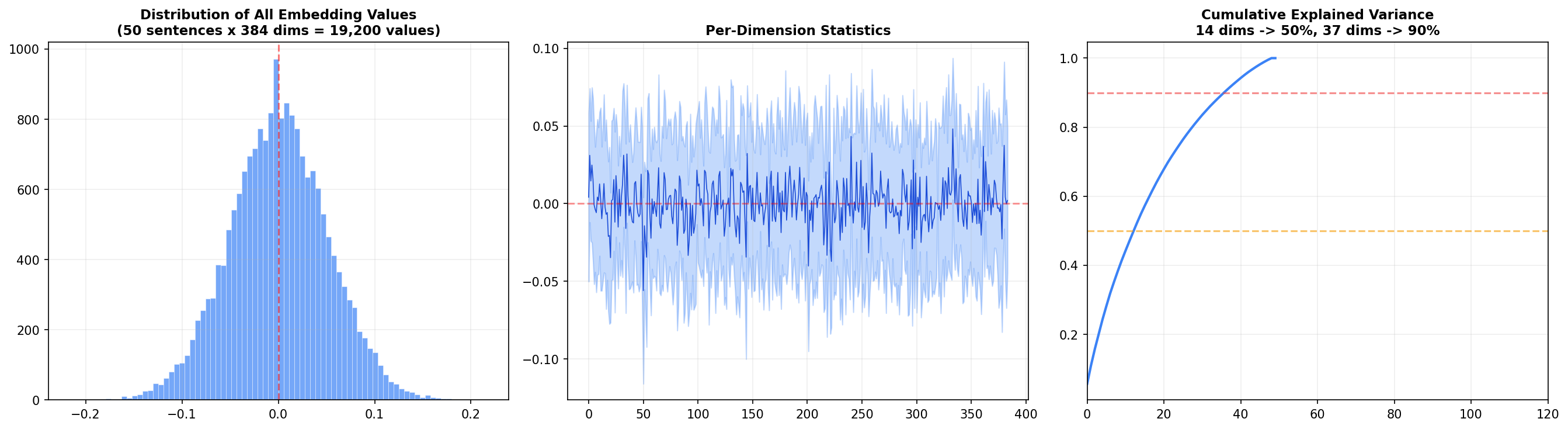
Left panel: The distribution of all 19,200 embedding values (50 sentences × 384 dims) is roughly normal and centered at zero. This is a consequence of L2 normalization — values cluster around zero with a standard deviation around 0.05.

Center panel: Each dimension's mean and standard deviation across the 50 sentences. Most dimensions oscillate near zero, but a handful show systematic biases — these are the dimensions that encode broad features like sentence length or overall sentiment.

Right panel: The cumulative explained variance — the big insight. 14 dimensions capture 50% of the total variance, and 37 dimensions capture 90%. That means 347 of the 384 dimensions contribute only 10% of the information. Why have all 384? Because that last 10% encodes subtle distinctions — the difference between "happy" and "joyful," or "argued" and "debated." For search and retrieval, those distinctions matter.

Semantic Similarity in Action

Visualizations are great, but the real test is whether the model can distinguish meaning from vocabulary. Here are four controlled pairs:

Sentence A                                    Sentence B                              Sim     Relation
────────────────────────────────────────────────────────────────────────────────────────────────────
The dog played in the park                    A canine ran through the green field    54.1%   ✓ SAME
The dog played in the park                    The stock market crashed yesterday       3.8%    ✗ DIFF
I love eating pizza and pasta                 Italian cuisine is my favorite food      61.6%   ✓ SAME
I love eating pizza and pasta                 The spaceship launched into orbit         9.0%    ✗ DIFF
She felt incredibly happy today               Joy radiated from her entire being       58.7%   ✓ SAME
She felt incredibly happy today               The computer needs a software update      6.5%    ✗ DIFF
Machine learning is transforming industries   AI and deep learning are reshaping biz   68.5%   ✓ SAME
Machine learning is transforming industries   The cat napped in the warm sunlight      -4.8%   ✗ DIFF

Every pair with shared meaning scores above 50%. Every pair with shared words but different meaning scores below 10%. The model even produces negative similarity for the ML-vs-cat pair — indicating the embeddings point in opposite directions. It's not just distinguishing; it's contrasting.

Across all 50 sentences, the model found these as its most similar and most different pairs:

MOST SIMILAR:
  53.2% — "Swimming is an excellent full-body workout"  ↔  "Regular exercise reduces heart disease risk"
  43.3% — "Fresh ingredients make the best meals"       ↔  "A balanced diet provides essential nutrients"
  42.8% — "DNA contains the genetic blueprint"          ↔  "Evolution explains the diversity of life"

MOST DIFFERENT:
  -12.9% — "Japanese sushi demands precise knife skills" ↔ "Paris is the city of love and romance"

The most similar pairs are genuinely related concepts across different vocabulary. The most different pair — sushi vs Paris — is almost comically unrelated, and the model correctly places them at opposite ends of the embedding space.

How to Use Embeddings in Practice

Once you have embeddings, you unlock a family of capabilities:

• Semantic search: Embed a query, find the nearest document embeddings. We built a complete search engine with this technique in our FAISS semantic search tutorial.
• Clustering: Group thousands of documents into topics without any labels — run k-means on the embeddings. Great for exploring unlabeled datasets.
• Classification: Train a simple classifier on top of embeddings instead of raw text. Embeddings already encode semantic features, so even logistic regression performs well.
• Duplicate detection: Find near-duplicate content by thresholding cosine similarity — catches paraphrased content that keyword matching misses.
• Recommendation: Recommend similar articles, products, or messages by finding items with the closest embeddings.
• RAG pipelines: Retrieve relevant context for LLMs by embedding your knowledge base and searching it at query time. See our full RAG chatbot tutorial for a complete implementation.

Choosing the Right Embedding Model

For this tutorial I used MiniLM because it's fast, small, and produces embeddings good enough to demonstrate all the concepts. For production semantic search, mpnet-base-v2 is the standard choice — it tops the Sentence Transformers benchmark for semantic similarity tasks.

Wrapping Up

Text embeddings are one of those rare concepts where the core idea is simple — similar meanings map to nearby points — but the implications are profound. Once you internalize that text can be converted to coordinates in a semantic space, you start seeing applications everywhere: search, clustering, recommendation, duplicate detection, retrieval.

The visualizations tell the story: PCA shows broad structure, t-SNE reveals tight clusters, heatmaps quantify pairwise similarity, and dimension analysis exposes how information is distributed. Together, they transform embeddings from a black box into something you can see, understand, and trust.

The complete code is below. Install the dependencies, drop it in a .py file, and start generating your own embeddings.

Further Reading:

• How to Build a Semantic Search Engine with FAISS — use embeddings for real-time search
• Building a Full-Stack RAG Chatbot — embeddings + LLMs in production
• Sentence Transformers Documentation — full model list, training guides

Just finished the article? Why not take your Python skills a notch higher with our Python Code Assistant? Check it out!

Comment panel