How to Extract Google Trends Data in Python

Get a head start on your coding projects with our Python Code Generator. Perfect for those times when you need a quick solution. Don't wait, try it today!

Google Trends is a website created by Google that analyzes the popularity of search queries on Google Search across almost every region, language, and category.

In this tutorial, you will learn how to extract Google Trends data using Pytrends, an unofficial library in Python, to extract almost everything available on the Google Trends website.

Here is the table of content:

• Getting Started
• Interest over Time
• Interest by Region
• Related Topics and Queries
• Trending Searches
• Conclusion

Getting Started

To get started, let's install the required dependencies:

$ pip install pytrends seaborn

We'll use Seaborn just for beautiful plots, nothing else:

from pytrends.request import TrendReq
import seaborn
# for styling
seaborn.set_style("darkgrid")

To begin with pytrends, you have to create a TrendReq object:

# initialize a new Google Trends Request Object
pt = TrendReq(hl="en-US", tz=360)

The hl parameter is the host language for accessing Google Trends, and tz is the timezone offset.

There are other parameters such as retries indicating the number of retrials if the request fails or using proxies by passing a list to proxies parameter.

Interest over Time

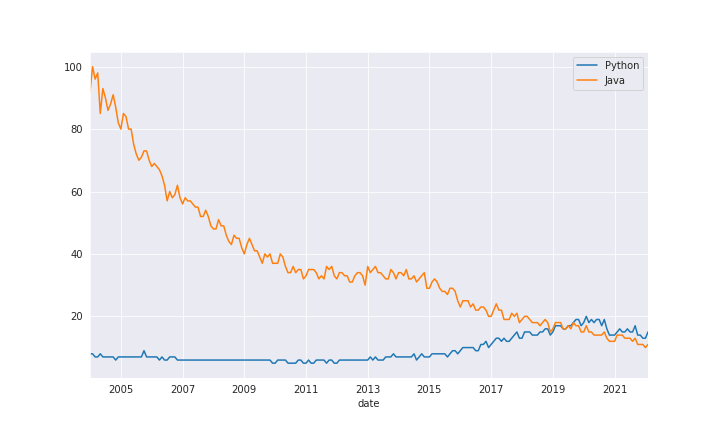
To get the relative number of searches of a list of keywords, we can use the interest_over_time() method after building the payload:

# set the keyword & timeframe
pt.build_payload(["Python", "Java"], timeframe="all")

# get the interest over time
iot = pt.interest_over_time()
iot

Output:

		Python	Java	isPartial
date			
2004-01-01	8	92	False
2004-02-01	8	100	False
2004-03-01	7	96	False
2004-04-01	7	98	False
2004-05-01	8	85	False
...	...	...	...
2021-10-01	14	11	False
2021-11-01	14	11	False
2021-12-01	13	11	False
2022-01-01	13	10	False
2022-02-01	15	11	True
218 rows × 3 columns

The values range from 0 (few or no searches) to 100 (maximum possible searches).

The build_payload() method accepts several parameters besides the keyword list:

• cat: You can specify the category ID; if a search query can mean more than one meaning, setting the category will remove the confusion. You can check this page for a list of category IDs or simply call pytrends.categories() method to retrieve them.
• geo: The two-letter country abbreviation to get searches of a specific country, such as US, FR, ES, DZ, etc. You can also get data for provinces by specifying additional abbreviations such as 'GB-ENG' or 'US-AL'.
• timeframe: It is the time range of the data we want to extract, 'all' means all the data that is available on Google since the beginning, you can pass specific datetimes, or the minus patterns such as 'today 6-m' will return the latest six months data, 'today 3-d' will return the latest three days, and so on. The default of this parameter is 'today 5-y' meaning the last five years.

Let's plot the relative search difference between Python and Java over time:

# plot it
iot.plot(figsize=(10, 6))

Output:

Alternatively, we can use the get_historical_interest() method which grabs hourly data. However, that's not useful if you're seeking long-term trends. It's suitable for short periods:

# get hourly historical interest
data = pt.get_historical_interest(
    ["data science"], 
    year_start=2022, month_start=1, day_start=1, hour_start=0,
    year_end=2022, month_end=2, day_end=10, hour_end=23,
)
data

We set the starting and ending date and time and retrieve the results. You can also pass cat and geo as mentioned earlier. Here is the output:

			data science	isPartial
date		
2022-01-01 00:00:00	28	False
2022-01-01 01:00:00	34	False
2022-01-01 02:00:00	42	False
2022-01-01 03:00:00	44	False
2022-01-01 04:00:00	52	False
...	...	...
2022-02-10 19:00:00	69	False
2022-02-10 20:00:00	70	False
2022-02-10 21:00:00	69	False
2022-02-10 22:00:00	73	False
2022-02-10 23:00:00	68	False
989 rows × 2 columns

If there's something quickly emerging, this method will definitely be helpful. Note that this method can cause Google to block your IP, as it grabs a lot of data if you specify an extended timeframe, so keep that in mind.

Interest by Region

Let's get the interest of a specific keyword by region:

# the keyword to extract data
kw = "python"
pt.build_payload([kw], timeframe="all")
# get the interest by country
ibr = pt.interest_by_region("COUNTRY", inc_low_vol=True, inc_geo_code=True)

We pass "COUNTRY" to the interest_by_region() method to get the interest by country. Other possible values are 'CITY' for city-level data, 'DMA' for Metro-level data, and 'REGION' for region-level data.

We set inc_low_vol to True so we include the low search volume countries, we also set inc_geo_code to True to include the geocode of each country.

Let's sort the countries by interest in Python:

# sort the countries by interest
ibr[kw].sort_values(ascending=False)

Output:

geoName
British Indian Ocean Territory    100
St. Helena                         38
China                              25
South Korea                        25
Singapore                          22
                                 ... 
Pitcairn Islands                    0
Guinea-Bissau                       0
São Tomé & Príncipe                 0
British Virgin Islands              0
Svalbard & Jan Mayen                0
Name: python, Length: 250, dtype: int64

You can also plot the top 10 if you wish, using ibr[kw].sort_values(ascending=False)[:10].plot.bar().

Related Topics and Queries

Another cool feature is to extract related topics of your keyword:

# get related topics of the keyword
rt = pt.related_topics()
rt[kw]["top"]

The related_topics() method returns a Python dictionary of each keyword; this dictionary has two dataframes, one for rising topics and one for overall top topics. Below is the output:

value	formattedValue		hasData	link						topic_mid	topic_title		topic_type
0	100		100	True	/trends/explore?q=/m/05z1_&date=all		/m/05z1_	Python			Programming language
1	7		7	True	/trends/explore?q=/m/01dlmc&date=all		/m/01dlmc	List			Abstract data type
2	6		6	True	/trends/explore?q=/m/06x16&date=all		/m/06x16	String			Computer science
3	6		6	True	/trends/explore?q=/m/020s1&date=all		/m/020s1	Computer file		Topic
4	5		5	True	/trends/explore?q=/m/0cv6_m&date=all		/m/0cv6_m	Pythons			Snake
5	3		3	True	/trends/explore?q=/m/0nk18&date=all		/m/0nk18	Associative array	Topic
6	3		3	True	/trends/explore?q=/m/026sq&date=all		/m/026sq	Data			Topic
...
20	2		2	True	/trends/explore?q=/m/021plb&date=all		/m/021plb	NumPy			Software
21	2		2	True	/trends/explore?q=/m/016r48&date=all		/m/016r48	Object			Computer science
22	2		2	True	/trends/explore?q=/m/0fpzzp&date=all		/m/0fpzzp	Linux			Operating system
23	1		1	True	/trends/explore?q=/m/0b750&date=all		/m/0b750	Subroutine		Topic
24	1		1	True	/trends/explore?q=/m/02640pc&date=all		/m/02640pc	Import			Topic

Or related search queries:

# get related queries to previous keyword
rq = pt.related_queries()
rq[kw]["top"]

Output:

query	value
0	python for	100
1	python list	97
2	python file	74
3	python string	73
4	monty python	44
5	install python	42
6	python if	41
7	python function	39
8	python download	34
9	python windows	33
10	python array	31
11	dictionary python	30
12	ball python	30
13	pandas	29
14	pandas python	29
15	python tutorial	26
16	python script	24
17	python class	23
18	python import	23
19	numpy	22
20	python set	22
21	python programming	21
22	python online	20
23	python time	19
24	python pdf	19

Also, there is the suggestions(keyword) method that returns the suggested search queries:

# get suggested searches
pt.suggestions("python")

Output:

[{'mid': '/m/05z1_', 'title': 'Python', 'type': 'Programming language'},
 {'mid': '/m/05tb5', 'title': 'Python family', 'type': 'Snake'},
 {'mid': '/m/0cv6_m', 'title': 'Pythons', 'type': 'Snake'},
 {'mid': '/m/01ny0v', 'title': 'Ball python', 'type': 'Reptiles'},
 {'mid': '/m/02_2hl', 'title': 'Python', 'type': 'Film'}]

Here is another example:

# another example of suggested searches
pt.suggestions("America")

Output:

[{'mid': '/m/09c7w0',
  'title': 'United States',
  'type': 'Country in North America'},
 {'mid': '/m/01w6dw',
  'title': 'American Express',
  'type': 'Credit card service company'},
 {'mid': '/m/06n3y', 'title': 'South America', 'type': 'Continent'},
 {'mid': '/m/03lq2', 'title': 'Halloween', 'type': 'Celebration'},
 {'mid': '/m/01yx7f',
  'title': 'Bank of America',
  'type': 'Financial services company'}]

Trending Searches

One more feature on Google trends is the ability to extract the current trending searches on each region:

# trending searches per region
ts = pt.trending_searches(pn="united_kingdom")
ts[:5]

Output:

0	Championship
1	Super Bowl
2	Sheffield United
3	Kodak Black
4	Atletico Madrid

Another alternative is realtime_trending_searches():

# real-time trending searches
pt.realtime_trending_searches()

Output:

title	entityNames
0	Jared Cannonier, Derek Brunson, Mixed martial ...	[Jared Cannonier, Derek Brunson, Mixed martial...
1	Christian Nodal, Belinda	[Christian Nodal, Belinda]
2	Vladimir Putin, Russia	[Vladimir Putin, Russia]
3	River Radamus, Slalom skiing, Giant slalom, Wi...	[River Radamus, Slalom skiing, Giant slalom, W...
4	California State University, Fullerton, Cal St...	[California State University, Fullerton, Cal S...
...	...	...
81	Javier Bardem, Minority group, Desi Arnaz, Aar...	[Javier Bardem, Minority group, Desi Arnaz, Aa...
82	Marvel Cinematic Universe, Thanos, Avengers: E...	[Marvel Cinematic Universe, Thanos, Avengers: ...
83	Siena Saints, College basketball, Rider Broncs...	[Siena Saints, College basketball, Rider Bronc...
84	Chicago Blackhawks, St. Louis Blues, National ...	[Chicago Blackhawks, St. Louis Blues, National...
85	New York Islanders, Calgary Flames, National H...	[New York Islanders, Calgary Flames, National ...
86 rows × 2 columns

Conclusion

Alright, you now know how to conveniently extract Google Trends data using Python and with the help of the pytrends library. You can check the Pytrends Github repository for more detailed information on the methods we've used in this tutorial.

You can get the complete code here.

Learn also: How to Extract Wikipedia Data in Python

Happy extracting ♥

Just finished the article? Why not take your Python skills a notch higher with our Python Code Assistant? Check it out!

Read Also

How to Extract Wikipedia Data in Python

Extracting data and searching in Wikipedia, getting article summaries, links, images and more using Wikipedia library in Python.

Visit →

How to Extract YouTube Data in Python

Scraping YouTube videos and extracting useful video information such as title, total views, publish date, video duration, tags, likes and dislikes and more in Python using requests_html and Beautiful Soup libraries.

Visit →

How to Get Geolocation in Python

Learn how to use GeoPy library to geocode physical addresses into latitude and longitude and vice versa; getting latitude and longitude from addresses, towns, cities and more in Python.

Visit →

Comment panel