Confused by complex code? Let our AI-powered Code Explainer demystify it for you. Try it out!
Introduction
A dataset with unequal classes is a popular data science challenge and an interesting interview question. This tutorial will show you how to effectively optimize your model and handle unbalanced data.
Classification issues such as spam filtering, credit card fraud detection, medical diagnosis problems such as skin cancer detection, and churn prediction are among the most prevalent areas where you may find unbalanced data.
Almost every dataset has an uneven class representation. It isn't an issue as long as the difference is negligible. However, many models fail to detect the minority classes when one or more classes are very uncommon.
This tutorial will assume a two-class issue (one majority class and one minority class).
Typically, we check the accuracy on the validation split to see how well our model is functioning. Nevertheless, when the data is skewed, accuracy might be deceptive.
Table of content:
- Introduction
- Data Description
- Encoding Categorical Variables
- Performing Data Visualization
- Running the Logistic Regression
- Dealing with Class Imbalance using Class Weight
- Dealing with Class Imbalance using Resampling
- Dealing with Class Imbalance using SMOTE
- Conclusion
Data Description
This data contains information about a video streaming service firm that wants to estimate whether or not a client would churn.
The CSV file has around 2000 rows and 16 columns. The dataset can be downloaded here.
Before we get started, let's install the necessary libraries for this tutorial:
$ pip install numpy sklearn imblearn pandas statsmodels seabornLet's install gdown for downloading the dataset automatically:
$ pip install --upgrade gdownDownloading the dataset:
$ gdown --id 12vfq3DYFId3bsXuNj_PhsACMzrLTfObsOutput:
Downloading...
From: https://drive.google.com/uc?id=12vfq3DYFId3bsXuNj_PhsACMzrLTfObs
To: /content/data_regression.csv
100% 138k/138k [00:00<00:00, 72.5MB/s]
Now we have everything ready, let's start by importing the necessary libraries:
import numpy as np
from sklearn.model_selection import train_test_split
from imblearn.over_sampling import SMOTE
from sklearn.utils import resample
import pandas as pd
from sklearn.linear_model import LogisticRegression
from sklearn.metrics import roc_auc_score, classification_report
from sklearn.metrics import confusion_matrix
from sklearn.linear_model import LogisticRegression
import statsmodels.api as sm
import seaborn as sns
from sklearn.preprocessing import OrdinalEncoder
Loading the dataset:
data=pd.read_csv("data_regression.csv")
# get the first 5 rows
data.head()
╔═══╤══════╤═════════════╤══════════╤════════╤═════╤═══════════════════════╤══════════════╤═════════════════╤═════════════════════╤════════════════════╤════════════════════╤═══════════════════════╤════════════════╤═══════════════════════╤════════════════════════╤═══════╗
║ │ year │ customer_id │ phone_no │ gender │ age │ no_of_days_subscribed │ multi_screen │ mail_subscribed │ weekly_mins_watched │ minimum_daily_mins │ maximum_daily_mins │ weekly_max_night_mins │ videos_watched │ maximum_days_inactive │ customer_support_calls │ churn ║
╠═══╪══════╪═════════════╪══════════╪════════╪═════╪═══════════════════════╪══════════════╪═════════════════╪═════════════════════╪════════════════════╪════════════════════╪═══════════════════════╪════════════════╪═══════════════════════╪════════════════════════╪═══════╣
║ 0 │ 2015 │ 100198 │ 409-8743 │ Female │ 36 │ 62 │ no │ no │ 148.35 │ 12.2 │ 16.81 │ 82 │ 1 │ 4.0 │ 1 │ 0.0 ║
╟───┼──────┼─────────────┼──────────┼────────┼─────┼───────────────────────┼──────────────┼─────────────────┼─────────────────────┼────────────────────┼────────────────────┼───────────────────────┼────────────────┼───────────────────────┼────────────────────────┼───────╢
║ 1 │ 2015 │ 100643 │ 340-5930 │ Female │ 36 │ 149 │ no │ no │ 294.45 │ 7.7 │ 33.37 │ 87 │ 3 │ 3.0 │ 2 │ 0.0 ║
╟───┼──────┼─────────────┼──────────┼────────┼─────┼───────────────────────┼──────────────┼─────────────────┼─────────────────────┼────────────────────┼────────────────────┼───────────────────────┼────────────────┼───────────────────────┼────────────────────────┼───────╢
║ 2 │ 2015 │ 100756 │ 372-3750 │ Female │ 36 │ 126 │ no │ no │ 87.30 │ 11.9 │ 9.89 │ 91 │ 1 │ 4.0 │ 5 │ 1.0 ║
╟───┼──────┼─────────────┼──────────┼────────┼─────┼───────────────────────┼──────────────┼─────────────────┼─────────────────────┼────────────────────┼────────────────────┼───────────────────────┼────────────────┼───────────────────────┼────────────────────────┼───────╢
║ 3 │ 2015 │ 101595 │ 331-4902 │ Female │ 36 │ 131 │ no │ yes │ 321.30 │ 9.5 │ 36.41 │ 102 │ 4 │ 3.0 │ 3 │ 0.0 ║
╟───┼──────┼─────────────┼──────────┼────────┼─────┼───────────────────────┼──────────────┼─────────────────┼─────────────────────┼────────────────────┼────────────────────┼───────────────────────┼────────────────┼───────────────────────┼────────────────────────┼───────╢
║ 4 │ 2015 │ 101653 │ 351-8398 │ Female │ 36 │ 191 │ no │ no │ 243.00 │ 10.9 │ 27.54 │ 83 │ 7 │ 3.0 │ 1 │ 0.0 ║
╚═══╧══════╧═════════════╧══════════╧════════╧═════╧═══════════════════════╧══════════════╧═════════════════╧═════════════════════╧════════════════════╧════════════════════╧═══════════════════════╧════════════════╧═══════════════════════╧════════════════════════╧═══════╝The function below will help in inspection and cleaning the data frame:
# check for the missing values and dataframes
def datainspection(dataframe):
  print("Types of the variables we are working with:")
  print(dataframe.dtypes)

  print("Total Samples with missing values:")

  print(data.isnull().any(axis=1).sum()) # null values

  print("Total Missing Values per Variable")
  print(data.isnull().sum())
  print("Map of missing values")
sns.heatmap(dataframe.isnull())datainspection(data)age int64
no_of_days_subscribed int64
multi_screen object
mail_subscribed object
weekly_mins_watched float64
minimum_daily_mins float64
maximum_daily_mins float64
weekly_max_night_mins int64
videos_watched int64
maximum_days_inactive float64
customer_support_calls int64
churn float64
dtype: object
Total Samples with missing values:
82
Total Missing Values per Variable
year 0
customer_id 0
phone_no 0
gender 24
age 0
no_of_days_subscribed 0
multi_screen 0
mail_subscribed 0
weekly_mins_watched 0
minimum_daily_mins 0
maximum_daily_mins 0
weekly_max_night_mins 0
videos_watched 0
maximum_days_inactive 28
customer_support_calls 0
churn 35
dtype: int64
Map of missing valuesWe will drop all the null values:
data = data.dropna() # cleaning up null valuesEncoding Categorical Variables
The OrdinalEncoder() class will be used to encode categorical features as an integer array:
# function for encoding categorical variables
def encode_cat(data, vars):
  ord_en = OrdinalEncoder()
  for v in vars:
    name = v+'_code' # add _code for encoded variables
    data[name] = ord_en.fit_transform(data[[v]])
    print('The encoded values for '+ v + ' are:')
    print(data[name].unique())
  return data
# check for the encoded variables
data = encode_cat(data, ['gender', 'multi_screen', 'mail_subscribed'])The encoded values for gender are:
[0. 1.]
The encoded values for multi_screen are:
[0. 1.]
The encoded values for mail_subscribed are:
[0. 1.]Performing Data Visualization
The below function will return a pairplot of all the variables in the dataset. The select_dtypes() function retrieves a subset of the columns in the DataFrame depending on the column types. We pass the columns to exclude as a list to the difference method:
def full_plot(data, class_col, cols_to_exclude):
  cols = data.select_dtypes(include=np.number).columns.tolist() # finding all the numerical columns from the dataframe
  X = data[cols] # creating a dataframe only with the numerical columns
  X = X[X.columns.difference(cols_to_exclude)] # columns to exclude
  X = X[X.columns.difference([class_col])]
  sns.pairplot(data, hue=class_col)
To display the pairplots, we must call the function above:
full_plot(data,class_col='churn', cols_to_exclude=['customer_id','phone_no', 'year'])We will let you perform this operation and see the result, as it takes a few seconds to minutes to finish.
Nevertheless, the function below will help us if we want to create plots for selective columns:
# function for creating plots for selective columns only
def selected_diagnotic(data,class_col, cols_to_eval):
  cols_to_eval.append(class_col)
  X = data[cols_to_eval] # only selective columns
  sns.pairplot(X, hue=class_col) # plot
selected_diagnotic(data, class_col='churn', cols_to_eval=['videos_watched', 'no_of_days_subscribed'])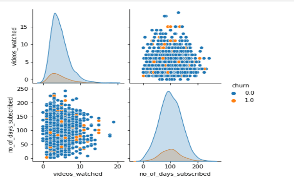
Running the Logistic Regression
The function below performs the logistic regression task using statsmodels, which is a Python module that supplies classes and methods for estimating a wide range of statistical models, performing statistical tests, and exploring statistical data.
Logit() is a method provided by statsmodels for performing logistic regression. It takes two inputs, y and X, and returns a Logit object.
After that, the model is fitted to the data. The table below provides a descriptive summary of the regression findings.
def logistic_regression(data, class_col, cols_to_exclude):
  cols = data.select_dtypes(include=np.number).columns.tolist()
  X = data[cols]
  X = X[X.columns.difference([class_col])]
  X = X[X.columns.difference(cols_to_exclude)] # unwanted columns

  y = data[class_col] # the target variable
  logit_model = sm.Logit(y,X)
  result = logit_model.fit() # fit the model
  print(result.summary2()) # check for summary
logistic_regression(data, class_col='churn', cols_to_exclude=['customer_id', 'phone_no', 'year'])Optimization terminated successfully.
Current function value: 0.336585
Iterations 7
Results: Logit
=======================================================================
Model: Logit Pseudo R-squared: 0.137
Dependent Variable: churn AIC: 1315.1404
Date: 2022-04-01 12:22 BIC: 1381.8488
No. Observations: 1918 Log-Likelihood: -645.57
Df Model: 11 LL-Null: -748.02
Df Residuals: 1906 LLR p-value: 7.1751e-38
Converged: 1.0000 Scale: 1.0000
No. Iterations: 7.0000
-----------------------------------------------------------------------
Coef. Std.Err. z P>|z| [0.025 0.975]
-----------------------------------------------------------------------
age -0.0208 0.0068 -3.0739 0.0021 -0.0340 -0.0075
customer_support_calls 0.4246 0.0505 8.4030 0.0000 0.3256 0.5237
gender_code -0.2144 0.1446 -1.4824 0.1382 -0.4979 0.0691
mail_subscribed_code -0.7529 0.1798 -4.1873 0.0000 -1.1053 -0.4005
maximum_daily_mins -3.7125 25.2522 -0.1470 0.8831 -53.2058 45.7809
maximum_days_inactive -0.7870 0.2473 -3.1828 0.0015 -1.2716 -0.3024
minimum_daily_mins 0.2075 0.0727 2.8555 0.0043 0.0651 0.3499
multi_screen_code 1.9511 0.1831 10.6562 0.0000 1.5923 2.3100
no_of_days_subscribed -0.0045 0.0018 -2.5572 0.0106 -0.0080 -0.0011
videos_watched -0.0948 0.0317 -2.9954 0.0027 -0.1569 -0.0328
weekly_max_night_mins -0.0169 0.0032 -5.3119 0.0000 -0.0231 -0.0107
weekly_mins_watched 0.4248 2.8619 0.1484 0.8820 -5.1844 6.0340Some of the concepts in the summary table are defined as follows:
- Iterations: The number of times the model iterates through the data, attempting to optimize the model. The maximum number of iterations executed by default is 33, beyond which the optimization fails. Some of the concepts in the summary table are defined as follows:
- coef: The coefficients of the regression equation's independent variables.
- Log-Likelihood: Natural logarithm of the MLE function. MLE is the process of determining the collection of parameters that results in the best fit.
- LL-Null: the model's log-likelihood value when no independent variable is included.
- Pseudo R-square: Value used to replace R-squared in the least-squares linear regression. It is the ratio of the null model's log-likelihood to the complete model's log-likelihood.
- P-value: The p-value refers to the hypothesis testing, and the lower the p-value, the greater the importance of the variable in the model.
The two functions below will help to prepare and run the model. The first function will handle the partition, and the second will display the classification report and the Area Under the Curve:
def prepare_model(data, class_col, cols_to_exclude):
  # Split in training and test set
  # Selecting only the numerical columns and excluding the columns we specified in the function
  cols = data.select_dtypes(include=np.number).columns.tolist()
  X = data[cols]
  X = X[X.columns.difference([class_col])]
  X = X[X.columns.difference(cols_to_exclude)]
  # Selecting y as a column
  y = data[class_col]
  return train_test_split(X, y, test_size=0.3, random_state=0) # perform train test split
def run_model(X_train, X_test, y_train, y_test):
# Fitting the logistic regression
logreg = LogisticRegression(random_state=13)
logreg.fit(X_train, y_train) # fit the model
# Predicting y values
y_pred = logreg.predict(X_test) # make predictions on th test data
logit_roc_auc = roc_auc_score(y_test, logreg.predict(X_test))
print(classification_report(y_test, y_pred)) # check for classification report
print("The area under the curve is:", logit_roc_auc) # check for AUC
return y_predX_train, X_test, y_train, y_test = prepare_model(data, class_col='churn', cols_to_exclude=['customer_id', 'phone_no', 'year'])
y_pred = run_model(X_train, X_test, y_train, y_test) precision recall f1-score support
0.0 0.90 0.98 0.94 513
1.0 0.47 0.13 0.20 63
accuracy 0.89 576
macro avg 0.69 0.55 0.57 576
weighted avg 0.85 0.89 0.86 576
The area under the curve is: 0.55To quote from sklearn:
- The precision is the ratio tp / (tp + fp), where tp is the number of true positives and fp is the number of false positives.
- The precision is intuitively the ability of the classifier not to label as positive a sample that is negative.
- The recall is the ratio tp / (tp + fn), where tp is the number of true positives and fn is the number of false negatives.
- The recall is intuitively the ability of the classifier to find all the positive samples.
- The F-beta score can be interpreted as a weighted harmonic mean of the precision and recall, where an F-beta score reaches its best value at 1 and worst score at 0.
It is worth noting that the F1 score is too low here.
Let's perform a confusion matrix. A confusion matrix, which illustrates each class's accurate and wrong predictions, is an exciting tool to analyze the outcome.
def confusion_m(y_test, y_pred):
  cm = confusion_matrix(y_test, y_pred)
  print(cm)
  tn, fp, fn, tp = cm.ravel()
  print("TN:", tn)
  print("TP:", tp)
  print("FN:", fn)
  print("FP:", fp)
## Call the function
confusion_m(y_test, y_pred)[[504 9]
[ 55 8]]
TN: 504
TP: 8
FN: 55
FP: 9The first column in the first row represents how many classes 0 were successfully predicted, while the second column tells how many classes 0 were accurately forecasted as 1.
For the minority class, the model mentioned above can correctly predict 8 out of 63 samples. Only nine forecasts were incorrect for the majority class. Therefore, the model is not excellent at predicting minority classes.
Dealing with Class Imbalance using Class Weight
Many Scikit-Learn classifiers have a class_weights parameter that may be set to balance or given a custom dictionary to specify how to prioritize the relevance of unbalanced data.
It is comparable to oversampling. Instead of actually oversampling (since a more extensive dataset would be computationally more costly), we may instruct the estimator to adjust how it calculates loss.
We can compel an estimator to learn using weights depending on how much relevance (weight) we assign to a particular class.
We have defined class_weight="balanced" to replicate the smaller class until we get the same number of samples as the larger one.
# class imbalance method 1
def run_model_bweights(X_train, X_test, y_train, y_test):
    logreg = LogisticRegression(random_state=13, class_weight='balanced') # define class_weight parameter
    logreg.fit(X_train, y_train) # fit the model
    y_pred = logreg.predict(X_test) # predict on test data
    logit_roc_auc = roc_auc_score(y_test, logreg.predict(X_test)) # ROC AUC score
    print(classification_report(y_test, y_pred))
    print("The area under the curve is:", logit_roc_auc) # AUC curve
run_model_bweights(X_train, X_test, y_train, y_test) precision recall f1-score support
0.0 0.96 0.75 0.84 513
1.0 0.27 0.78 0.40 63
accuracy 0.75 576
macro avg 0.62 0.76 0.62 576
weighted avg 0.89 0.75 0.79 576
The area under the curve is: 0.76We can note a slight improvement in recall and F1 score. Let's continue by assigning more weight to the majority class (Random weight) and see what happens:
# class imbalance method 2
def run_model_aweights(X_train, X_test, y_train, y_test, w):
    logreg = LogisticRegression(random_state=13, class_weight=w) # define class_weight parameter
    logreg.fit(X_train, y_train) # fit the model
    y_pred = logreg.predict(X_test) # predict on test data
    logit_roc_auc = roc_auc_score(y_test, logreg.predict(X_test))  # ROC AUC score
    print(classification_report(y_test, y_pred))
    print("The area under the curve is: %0.2f"%logit_roc_auc)  # AUC curve
run_model_aweights(X_train,X_test,y_train,y_test,{0:90, 1:10}) precision recall f1-score support
0.0 0.89 1.00 0.94 513
1.0 1.00 0.02 0.03 63
accuracy 0.89 576
macro avg 0.95 0.51 0.49 576
weighted avg 0.90 0.89 0.84 576
The area under the curve is: 0.51We note a drastic drop with F1-score. So we must give more weight to the minority class instead. Minority classes must be offered more weight to suggest that the model should prioritize these classes. We must reduce the prominence of the majority classes by assigning lower weights to them.
Dealing with Class Imbalance using Resampling
This can be achieved by importing the resample module from scikit-learn. sklearn.resample does not add more data points to the datasets. Instead, it does a random resampling (with/without replacement) of your dataset.
This equalization approach prevents the machine learning model from prioritizing the majority class in the dataset:
# class imbalance method 3
def adjust_imbalance(X_train, y_train, class_col):
  X = pd.concat([X_train, y_train], axis=1)
  # separate the 2 classes. Here we divide majority and minority classes
  class0 = X[X[class_col] == 0]
  class1 = X[X[class_col] == 1]
  # Case 1 - bootstraps from the minority class
  if len(class1)<len(class0):
    resampled = resample(class1,
                              replace=True, # Upsampling with replacement
                              n_samples=len(class0), ## Number to match majority class
                              random_state=10)
    resampled_data = pd.concat([resampled, class0]) ## # Combination of majority and upsampled minority class
  # Case 1 - resamples from the majority class
  else:
    resampled = resample(class1,
                              replace=False, ## false instead of True like above
                              n_samples=len(class0),
                              random_state=10)
    resampled_data = pd.concat([resampled, class0])
  return resampled_data
## Call the function
resampled_data = adjust_imbalance(X_train, y_train, class_col='churn')X_train, X_test, y_train, y_test = prepare_model(resampled_data, class_col='churn', cols_to_exclude=['customer_id', 'phone_no', 'year'])
run_model(X_train, X_test, y_train, y_test) precision recall f1-score support
0.0 0.69 0.75 0.72 339
1.0 0.74 0.68 0.71 353
accuracy 0.71 692
macro avg 0.71 0.71 0.71 692
weighted avg 0.71 0.71 0.71 692
The area under the curve is: 0.71We note an improvement in the F1 score.
Dealing with Class Imbalance using SMOTE
SMOTE (Synthetic Minority Oversampling Technique) is a technique for creating elements for the minority class based on those that currently exist.
It operates by selecting a point at random from the minority class and calculating the k-nearest neighbors for that point.
The synthetic points are the points that are inserted between the specified point and its neighbors. SMOTE algorithm is implemented according to the following steps:
- Select an input vector from the minority class.
- Find its k closest neighbors (k neighbors is an input to the
SMOTE()method). - Select one of these neighbors and insert a synthetic point somewhere on the line connecting the point under consideration and its selected neighbor.
- Repeat the process until the data is balanced.
def prepare_data_smote(data,class_col,cols_to_exclude):
  # Synthetic Minority Oversampling Technique.
  # Generates new instances from existing minority cases that you supply as input.
  cols = data.select_dtypes(include=np.number).columns.tolist()
  X = data[cols]
  X = X[X.columns.difference([class_col])]
  X = X[X.columns.difference(cols_to_exclude)]
  y = data[class_col]
  X_train, X_test, y_train, y_test = train_test_split(X, y, test_size=0.3, random_state=0)
  sm = SMOTE(random_state=0, sampling_strategy=1.0)
  # run SMOTE on training set only
  X_train, y_train = sm.fit_resample(X_train, y_train)
  return X_train, X_test, y_train, y_test
X_train, X_test, y_train, y_test = prepare_data_smote(data,class_col='churn', cols_to_exclude=['customer_id', 'phone_no', 'year'])
run_model(X_train, X_test, y_train, y_test) precision recall f1-score support
0.0 0.96 0.75 0.84 513
1.0 0.26 0.71 0.38 63
accuracy 0.75 576
macro avg 0.61 0.73 0.61 576
weighted avg 0.88 0.75 0.79 576
The area under the curve is: 0.73Conclusion
An unbalanced dataset does not necessarily imply that the two classes are unpredictable.
Though most algorithms are intended to function with equal class distribution, up-sampling (e.g., SMOTE) is not the sole method for dealing with class imbalance. In the case of logistic regression and many other machine learning models, class weights may be modified to weight model error according to class distribution.
You can check the Colab notebook here.
Learn also: Credit Card Fraud Detection in Python.
Happy learning ♥
Want to code smarter? Our Python Code Assistant is waiting to help you. Try it now!
View Full Code Assist My Coding


Got a coding query or need some guidance before you comment? Check out this Python Code Assistant for expert advice and handy tips. It's like having a coding tutor right in your fingertips!