Unlock the secrets of your code with our AI-powered Code Explainer. Take a look!
Many have already stated that data is the new oil of the 21st century, from which many fields have emerged and created such as Data Science, Data Mining, Data Engineering and Big Data.
Whether it's in Physics, Medicine, Biology or Social Media, all of those generate data constantly which are stored, preprocessed and analyzed in the aim to extract valuable conclusions for accurate decision makings.
The financial market, known with its dynamic momentum due to the law of Demand/Supply and other economical factors, is also a place where data is tremendously produced. Analyzing stock prices, whether you are trading CFD (Contract For Difference), Futures or commodities, whatever broker you are using, it is highly recommended and even fundamental to maximize your gains while performing trading.
This tutorial will allow you to grasp a general idea on handling stock prices using Python, understand the candles prices format (OHLC), and plot them using Candlestick charts. You will also learn to use many technical indicators using stockstats library.
For this tutorial, you will need to install:
pip install pandas-datareader yfinance mpl-finance stockstatsImporting Data from Yahoo Finance API
To import the stock prices data, we need to specify the symbol of the Market Index or Share, in this example, we will import data from S&P 500 and AAPL.
Note: S&P500 is a Market Index, which is a metric to track the performance of a set of companies included in this index. For instance, S&P which includes the top 500 stocks in the USA, NASDAQ related to the Top IT-based companies, the GER30 concerns the top 30 stocks in Germany, etc.
The below code is responsible for importing stock prices of AAPL:
# import AAPL stock price
df_aapl = pdr.get_data_yahoo("AAPL", start="2019-01-01", end="2019-09-30")
To import SPY (SPDR S&P 500 Trust ETF):
# import SPY stock price
df_spy = pdr.get_data_yahoo("SPY", start="2019-01-01", end="2019-09-30")
Here is how it looks:
df_spy.head()Output:
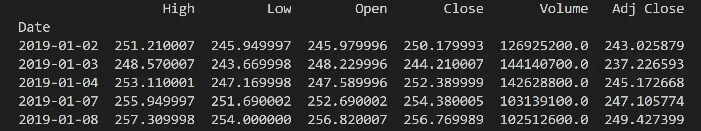
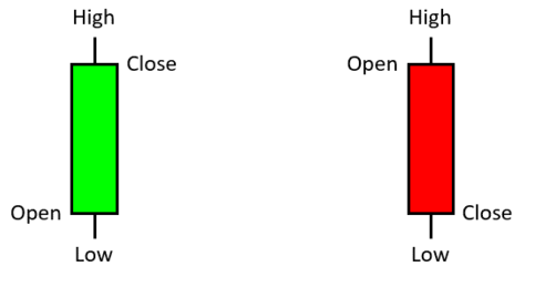
A candle in financial market is presented under the format OHLC which stands for "Open-High-Low-Close":
- Open: is the price of a stock when a time resolution started (1m, 30m, hourly, daily, etc)
- High: is the highest price reached from the beginning to the end of candle.
- Low: is the lowest price reached from the beginning to the end of candle.
- Close: is the price of a stock when a time resolution finishes.
We distinguish two types of trading operations when trading in the financial stock markets: Long (Buy) and Short (Sell).
Plotting Stock Prices
In this section, we will use matplotlib and mpl_finance libraries to plot the stock prices of AAPL. First, we will plot the Open-High-Low-Close prices separately:
df_aapl[["Open", "High", "Low", "Close"]].plot()
plt.show()
Output:
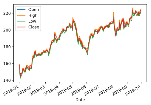
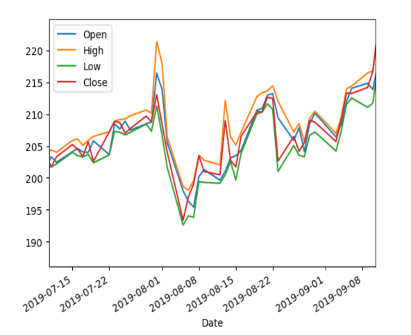
The figure in the left side shows the result of executing the above code, while the right figure is a zoomed region of the right figure.
We can clearly see in the zoomed region that the high prices (orange plot) is the upper bound, while the low prices (green plot) is the lower bound which illustrates the definition of the OHLC format mentioned in the previous section of the tutorial.
But as you may have already noticed, the plot is somehow difficult to read due to being charged, we will instead represent the OHLC in a form of a candlestick:
fig = plt.figure(figsize=(10, 10))
ax = plt.subplot()

plot_data = []
for i in range(150, len(df_aapl)):
    row = [
        i,
        df_aapl.Open.iloc[i],
        df_aapl.High.iloc[i],
        df_aapl.Low.iloc[i],
        df_aapl.Close.iloc[i],
    ]
    plot_data.append(row)
candlestick_ohlc(ax, plot_data)
plt.show()
Output:
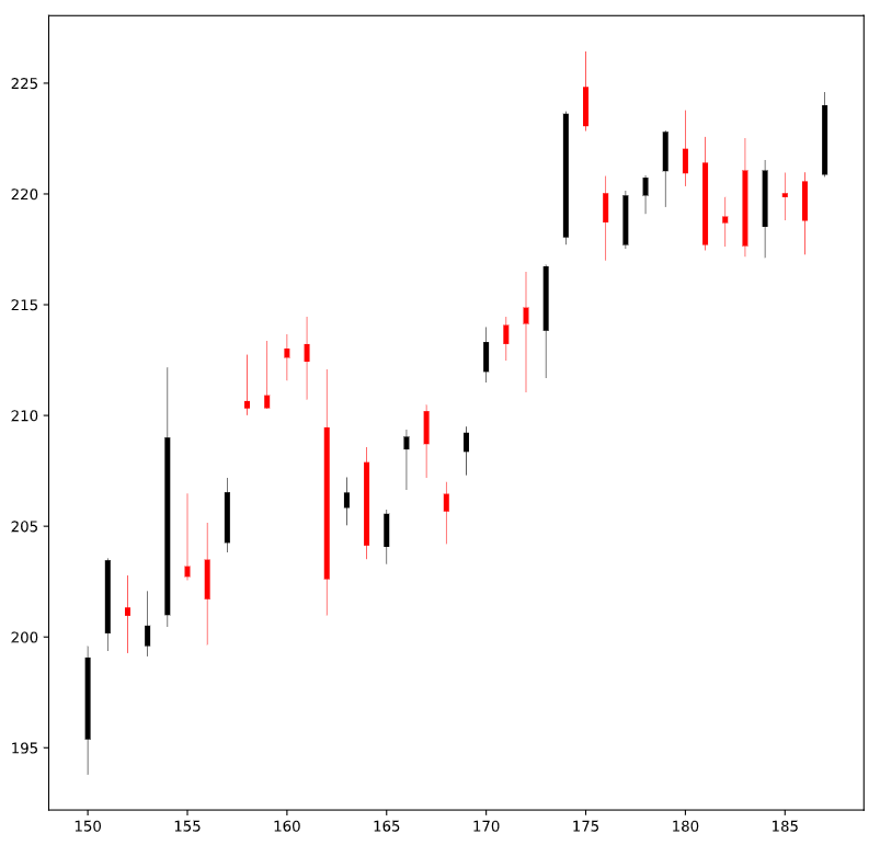 Here is how a candlestick is structured:
Financial Technical Indicators
In finance, and since we are handling numerical data, relying on various indicators will have a better view movements of the stock prices in addition to detecting trends which are very important in case we aim to do long-term trading/investment on a given stock.
From the stockstats library we will import StockDataFrame, which is a class that receives as an attribute a pandas DataFrame sorted by time and includes the columns Open-Close-High-Low in this order:
from stockstats import StockDataFrame

stocks = StockDataFrame.retype(df_aapl[["Open", "Close", "High", "Low", "Volume"]])
Simple Moving Average (SMA)
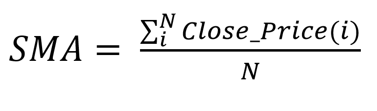
Simple Moving Average is an indicator which smoothens the stock prices plot, by computing the mean of the prices over a period of time. This will allow us to better visualize the trends directions (up or down).
The formula of SMA is shown in the following figure:
Plotting SMA:
plt.plot(stocks["close_10_sma"], color="b", label="SMA")
plt.plot(df_aapl.Close, color="g", label="Close prices")
plt.legend(loc="lower right")
plt.show()
Output:
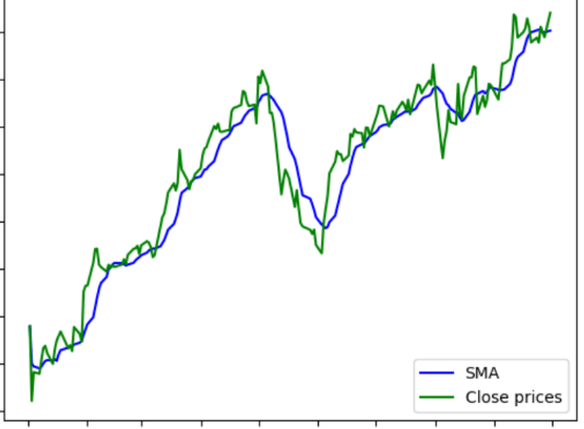 To compute the SMA, we specify the attribute under the following format:
Column_Period_Indicator
In our case, we are concerned about the Close prices within a period of 10 and the indicator is SMA, so the result is close_10_sma.
Exponential Moving Average (EMA)
Unlike the SMA, which gives equal weights to all prices whether the old or new ones, the Exponential Moving Average emphasizes on the last (most recent) prices by attributing to them a greater weight, this makes the EMA an indicator which detects trends faster than the SMA.
The formula of EMA is the following:
![]()
Plotting EMA:
plt.plot(stocks["close_10_sma"], color="b", label="SMA") # plotting SMA
plt.plot(stocks["close_10_ema"], color="k", label="EMA")
plt.plot(df_aapl.Close, color="g", label="Close prices") # plotting close prices
plt.legend(loc="lower right")
plt.show()
Output:
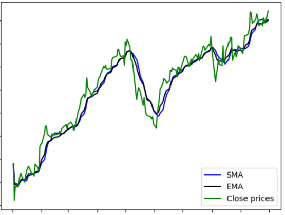
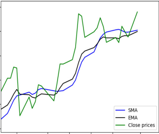
The left figure is the result of plotting the close prices, SMA and EMA, while the right figure is a zooming in a part of the original plot.
In the zoom figure, we can clearly observe that indeed EMA responds faster to the change of trends and gets closer to them.
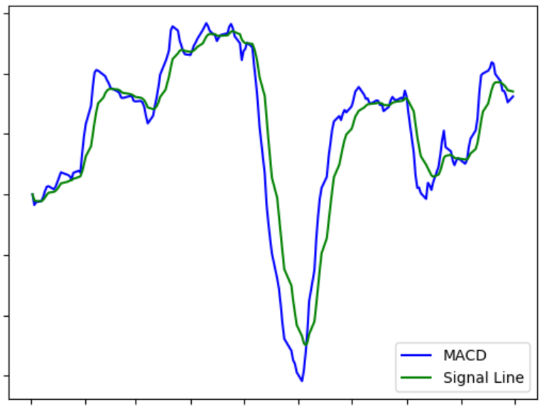
Moving Average Convergence/Divergence (MACD)
Moving Average Convergence/Divergence is a trend-following momentum indicator. This Indicator can show changes in the speed of price movement and traders use it to determine the direction of a trend.
The MACD is calculated by subtracting the 26-period Exponential Moving Average (EMA) from the 12-period EMA. A nine-day EMA of the MACD is called “Signal Line”, which is then plotted with the MACD.
When MACD crosses below the Signal Line it is an indicator to start doing short (Sell) operations. And when it crosses above it, it is an indicator to start doing long (Buy) operations:
plt.plot(stocks["macd"], color="b", label="MACD")
plt.plot(stocks["macds"], color="g", label="Signal Line")
plt.legend(loc="lower right")
plt.show()
Output:
That's it! There are many indicators offered by stockstats that anyone can explore, it can be plotted the same way the above mentioned ones.
Conclusion
In this tutorial, you:
- Learned how to import financial data using Pandas DataReader and yfinance libraries.
- Understood financial notations and definitions.
- Got familiar with the OHLC notation.
- Learned how to plot candlestick charts using mpl_finance library.
- Learned the importance of financial indicators and implemented some of them using the stockstats library.
If you want an in depth course which dives into more details in algorithmic trading, I would suggest you take Learn Algorithmic Trading with Python course, it is recommended by Investopedia, check it out!
Check the next tutorial in which you learn how to trade with FXCM Broker in Python.
Learn also: How to Predict Stock Prices in Python using TensorFlow 2 and Keras.
Happy Learning ♥
Just finished the article? Now, boost your next project with our Python Code Generator. Discover a faster, smarter way to code.
View Full Code Create Code for Me


Got a coding query or need some guidance before you comment? Check out this Python Code Assistant for expert advice and handy tips. It's like having a coding tutor right in your fingertips!