Unlock the secrets of your code with our AI-powered Code Explainer. Take a look!
Introduction
Logistic regression is a probabilistic model used to describe the probability of discrete outcomes given input variables. Despite the name, logistic regression is a classification model, not a regression model. In a nutshell, logistic regression is similar to linear regression except for categorization.
It computes the probability of the result using the sigmoid function. Because of the non-linear transformation of the input variable, logistic regression does not need linear correlations between input and output variables.
This tutorial focus on developing a logistic regression model for forecasting customer attrition in PyTorch.
What is a Logistic Regression
Although the method's name includes the term "regression", it is essentially a supervised machine learning technique designed to handle classification issues. It is due to the algorithm's usage of the logistic function, which ranges from 0 to 1.
As a result, we can use logistic regression to forecast the likelihood that a single feature variable (X) belongs to a specific category (Y).
Logistic regression has many similarities with linear regression, albeit linear regression is used to predict numerical values rather than classification issues. Both strategies use a line to depict the target variable.
Linear regression fits a line to the data to predict a new quantity, while logistic regression fits a line to separate the two classes optimally.
The Sigmoid Function
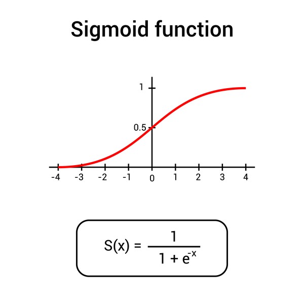
To understand what logistic regression is and how it works, you must first grasp the sigmoid function and the natural logarithm function.
This picture depicts the S-shaped curve of a variable for x values ranging from 0 to 1:
 Source: DepositPhotos
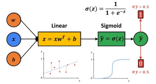
Throughout most of its domain, the sigmoid function has values that are extremely near to 0 or 1. Because of this, it is appropriate for use in binary classification problems. Take a look at the graphic below to see how the logistic regression model is represented:
Source: datahacker
As you can see, we'll start by computing the output of a linear function, z. The sigmoid function will take this output z as input. Following that, for computed z, we will generate the prediction ŷ, which z will determine. If z is a significant positive number, then ŷ will be near one.
On the other hand, if z has a significantly negative number, ŷ will be close to zero.
Consequently, ŷ will always be in the range from 0 to 1. Using a threshold value of 0.5 is a straightforward technique to categorize the prediction ŷ.
If our forecast is more extensive than 0.5, we assume ŷ equals 1.
Otherwise, we will suppose that ŷ is equal to zero. When we apply logistic regression, our objective is to attempt to calculate the parameters w and b so that ŷ becomes a decent estimate of the likelihood of ŷ=1.
Data Description
The dataset used in this study provides information on customer attrition based on various variables. The dataset has 2000 rows and 15 features that may be used to predict churn. It can be downloaded here.
Related: Customer Churn Prediction: A Complete Guide in Python.
Let's install the dependencies of this tutorial:
$ pip install matplotlib numpy pandas scikit_learn==1.0.2 torch==1.10.1To automatically download the dataset, we can use gdown:
$ pip install --upgrade gdown
$ gdown --id 12vfq3DYFId3bsXuNj_PhsACMzrLTfObs
Let's get started:
import pandas as pd
import numpy as np
import torch
import torch.nn as nn
from sklearn.utils import resample
from sklearn import preprocessing
from sklearn.preprocessing import StandardScaler
from sklearn.model_selection import train_test_split
from warnings import filterwarnings
filterwarnings('ignore')
Let's read the data, drop the year, customer_id, phone_no columns, and look at the shape of the data:
#reading data
data = pd.read_csv("data_regression.csv")
##The dimension of the data is seen, and the output column is checked to see whether it is continuous or discrete.
##In this case, the output is discrete, so a classification algorithm should be applied.
data = data.drop(["year", "customer_id", "phone_no"], axis=1)
print(data.shape)         # Lookiing the shape of the data
print(data.columns)       # Looking how many columns data has
data.dtypes
data.head()
Null Value Treatment
If we have null values, we need to work on that before feeding it to our model:
data.isnull().sum()gender 24
age 0
no_of_days_subscribed 0
multi_screen 0
mail_subscribed 0
weekly_mins_watched 0
minimum_daily_mins 0
maximum_daily_mins 0
weekly_max_night_mins 0
videos_watched 0
maximum_days_inactive 28
customer_support_calls 0
churn 35
dtype: int64final_data = data.dropna() # Dropping the null valuesData Sampling
Let us sample the data as our data is highly imbalanced. Upsampling and Downsampling have been used for minority and majority classes of the output. Finally, the data is concatenated for further processing:
final_data["churn"].value_counts()
# let us see how many data is there in each class for deciding the sampling data number
0.0 1665
1.0 253
Name: churn, dtype: int64Data Splitting
First, we need to split the data frame into separate classes before sampling:
data_majority = final_data[final_data['churn']==0] #class 0
data_minority = final_data[final_data['churn']==1] #class 1
#upsampling minority class
data_minority_upsampled = resample(data_minority, replace=True, n_samples=900, random_state=123)
 #downsampling majority class
data_majority_downsampled = resample(data_majority, replace=False, n_samples=900, random_state=123)
#concanating both upsampled and downsampled class
## Data Concatenation:  Concatenating the dataframe after upsampling and downsampling
#concanating both upsampled and downsampled class
data2 = pd.concat([data_majority_downsampled, data_minority_upsampled])
## Encoding Catagoricals:  We need to encode the categorical variables before feeding it to the model
data2[['gender', 'multi_screen', 'mail_subscribed']]
#label encoding categorical variables
label_encoder = preprocessing.LabelEncoder()
data2['gender']= label_encoder.fit_transform(data2['gender'])
data2['multi_screen']= label_encoder.fit_transform(data2['multi_screen'])
data2['mail_subscribed']= label_encoder.fit_transform(data2['mail_subscribed'])
## Lets now check again the distribution of the oputut class after sampling
data2["churn"].value_counts()
0.0 900
1.0 900
Name: churn, dtype: int64In the following code, we deal with scaling, splitting the training and testing sets, and separation of dependent and independent variables:
#indenpendent variable
X = data2.iloc[:,:-1]
## This X will be fed to the model to learn params
#scaling the data
sc = StandardScaler()         # Bringing the mean to 0 and variance to 1, so as to have a non-noisy optimization
X = sc.fit_transform(X)
X = sc.transform(X)
## Keeping the output column in a separate dataframe
data2 = data2.sample(frac=1).reset_index(drop=True) ## Shuffle the data frame and reset index
n_samples, n_features = X.shape ## n_samples is the number of samples and n_features is the number of features
#output column
Y = data2["churn"]
#output column
Y = data2["churn"]
##Data Splitting:
## The data is processed, so now we can split the data into train and test to train the model with training data and test it later from testing data.
#splitting data into train and test
X_train, X_test, y_train, y_test = train_test_split(X, Y, test_size=0.30, random_state=42, stratify = Y)
print((y_train == 1).sum())
print((y_train == 0).sum())
630
630Let's print the type of train and test set:
print(type(X_train))
print(type(X_test))
print(type(y_train.values))
print(type(y_test.values))
<class 'numpy.ndarray'>
<class 'numpy.ndarray'>
<class 'numpy.ndarray'>
<class 'numpy.ndarray'>Converting them to tensors as PyTorch works on, we will use the torch.from_numpy() method:
X_train = torch.from_numpy(X_train.astype(np.float32))
X_test = torch.from_numpy(X_test.astype(np.float32))
y_train = torch.from_numpy(y_train.values.astype(np.float32))
y_test = torch.from_numpy(y_test.values.astype(np.float32))
Making output vector Y as a column vector for matrix multiplications, we perform this change using the view operation as shown in the below code:
y_train = y_train.view(y_train.shape[0], 1)
y_test = y_test.view(y_test.shape[0], 1)
Activation Function
We use activation functions to represent the dynamic interaction in linear data. Here, we utilize a sigmoid activation function. We've picked the sigmoid function since it will limit the value from 0 to 1. Activation functions aid in introducing non-linearity into a neuron's output, which improves accuracy, computing efficiency, and convergence speed.
Activation functions should be differentiable and fast converging with respect to the weights.
Sigmoid disadvantages:
- Vanishing Gradient during the backpropagation stage of a neural network (especially RNNs).
- Because of its exponential nature, it is computationally expensive.
To quote from this paper: "The main activation function that was widely used is the Sigmoid function. However, when the Rectifier Linear Unit (ReLU) (Nair & Hinton, 2010) was introduced, it soon became a better replacement for the Sigmoid function due to its positive impact on the different machine learning tasks. While using Sigmoid and working on shallower layers doesn’t give any problem, some issues arise when the architecture becomes deeper because the derivative terms that are less than 1 will be multiplied by each other many times that the values will become smaller. and smaller until the gradient tends towards zero hence vanishing. On the other hand, if the values are bigger than one, the opposite happens, with numbers being multiplied becoming bigger and bigger until they tend to infinity and explode the gradient. A good solution would be to keep the values to 1 so even when they are multiplied, they don’t change. This is exactly what ReLU does: it has gradient 1 for positive inputs and 0 for negative ones.."
Model Building: Creating Logistic Regression model in Pytorch
Below is the responsible code for building the Logistic Regression model in PyTorch:
#logistic regression class
class LogisticRegression(nn.Module):
    def __init__(self, n_input_features):
        super(LogisticRegression, self).__init__()
        self.linear = nn.Linear(n_input_features, 1)

    #sigmoid transformation of the input
    def forward(self, x):
        y_pred = torch.sigmoid(self.linear(x))
        return y_pred
You must declare the layers in your model in the __init__() method. We have used linear layers, which are specified using the torch.nn module. The layer may be given any name, such as self.linear (in our case). I've declared one linear layer because that's logistic regression.
The syntax is: torch.nn.Linear(in_features, out_features, bias=True)
The forward() method is in charge of conducting the forward pass/propagation. The input is routed via the previously established layer, and the output of that layer is sent via the sigmoid activation function.
Let's initialize the model:
lr = LogisticRegression(n_features)Model Compiling
Let us define the number of epochs and the learning rate we want our model for training. As the data is binary, we will use Binary Cross Entropy as the loss function used to optimize the model using an SGD optimizer.
BCE Loss
We will also utilize the loss (error) function L to assess our algorithm's performance. Remember that the loss function is only applied to one training sample, and the most generally employed loss function is a squared error. However, the squared error loss function in logistic regression is not the best option. It produces an optimization problem that is not convex, and the gradient descent approach may not converge optimally. We will apply the BCE loss to hopefully reach the global optimum.
BCE loss stands for Binary Cross-Entropy loss and is often used in binary classification instances.
It is worth noting that when using the BCE loss function, the node's output should be between (0–1). For this, we'll need to employ an appropriate optimizer. We chose SGD, or Stochastic Gradient Descent, a regularly used optimizer. Other optimizers include Adam, Lars, and others.
You should provide model parameters and learning rate as input to the optimizer. SGD chooses one data point at random from the whole data set at each iteration to minimize computations drastically.
It is also usual to sample a tiny number of data points rather than just one at each step (often referred to as mini-batch gradient descent). Mini-batch attempts to balance gradient descent's efficiency and SGD's speed.
Learning Rate
The learning rate is an adjustable hyperparameter used in neural network training with a bit of positive value, often from 0.0 to 0.1. Lower learning rates need more training epochs because of the more minor changes in the weights with each update, while more excellent learning rates produce quick changes and require fewer training epochs.
A high learning rate might lead the model to converge too rapidly on a poor solution, while a low learning rate can cause the process to stall. Using the learning rate schedules, you may change the learning rate as the training progresses.
It adjusts the learning rate based on a predefined schedule, such as time-based, step-based, or exponential.
We may create a learning rate schedule to update the learning rate throughout training based on a predefined rule. The most common learning rate scheduler is a step decay, which reduces the learning rate by a certain percentage after a certain number of training epochs. Finally, we can say that a learning rate schedule is a predetermined structure for adjusting the learning rate across epochs or iterations as training occurs.
The following are two of the most prevalent strategies for learning rate schedules:
- Learning rate decay: It occurs when we choose an initial learning rate and then progressively lower it in compliance with a scheduler.
- Constant learning rate: As the name implies, we set a learning rate and do not vary it throughout training.
Note: The learning rate is a hyperparameter that should be tweaked. Instead of using a constant learning rate, we might start with a higher value of LR and then gradually decrease it after a specific number of rounds. It allows us to have quicker convergence at first while lowering the risks of overshooting the loss.
In PyTorch, we may utilize multiple schedulers from the optim package. You can follow this link to see how you can adjust the learning rate of a neural network using PyTorch. Let's define the parameters, the loss and the optimizer:
num_epochs = 500
# Traning the model for large number of epochs to see better results
learning_rate = 0.0001
criterion = nn.BCELoss()
# We are working on lgistic regression so using Binary Cross Entropy
optimizer = torch.optim.SGD(lr.parameters(), lr=learning_rate)
# Using ADAM optimizer to find local minima
Tracking the training process:
for epoch in range(num_epochs):
    y_pred = lr(X_train)
    loss = criterion(y_pred, y_train)
    loss.backward()
    optimizer.step()
    optimizer.zero_grad()
    if (epoch+1) % 20 == 0:
        # printing loss values on every 10 epochs to keep track
        print(f'epoch: {epoch+1}, loss = {loss.item():.4f}')
epoch: 20, loss = 0.8447
epoch: 40, loss = 0.8379
epoch: 60, loss = 0.8316
epoch: 80, loss = 0.8257
epoch: 100, loss = 0.8203
epoch: 120, loss = 0.8152
epoch: 140, loss = 0.8106
epoch: 160, loss = 0.8063
epoch: 180, loss = 0.8023
epoch: 200, loss = 0.7986
epoch: 220, loss = 0.7952
epoch: 240, loss = 0.7920
epoch: 260, loss = 0.7891
epoch: 280, loss = 0.7863
epoch: 300, loss = 0.7838
epoch: 320, loss = 0.7815
epoch: 340, loss = 0.7793
epoch: 360, loss = 0.7773
epoch: 380, loss = 0.7755
epoch: 400, loss = 0.7737
epoch: 420, loss = 0.7721
epoch: 440, loss = 0.7706
epoch: 460, loss = 0.7692
epoch: 480, loss = 0.7679
epoch: 500, loss = 0.7667Here, the first forward pass happens. Next, the loss is calculated. When loss.backward() is called, it computes the loss gradient with respect to the weights (of the layer). The weights are then updated by calling optimizer.step(). After this, the weights have to be emptied for the next iteration. So the zero_grad() method is called.
The above code prints the loss at each 20th epoch.
Model Performance
Let us finally see the model accuracy:
with torch.no_grad():
    y_predicted = lr(X_test)
    y_predicted_cls = y_predicted.round()
    acc = y_predicted_cls.eq(y_test).sum() / float(y_test.shape[0])
    print(f'accuracy: {acc.item():.4f}')
accuracy: 0.5093We have to use torch.no_grad() here. The goal is to omit the gradient computation over the weights. So, anything I put within this loop will not modify the weights and thus will not disrupt the backpropagation process.
We can also see the precision, recall, and F1 score using the classification report:
#classification report
from sklearn.metrics import classification_report
print(classification_report(y_test, y_predicted_cls))
precision recall f1-score support
0.0 0.51 0.62 0.56 270
1.0 0.51 0.40 0.45 270
accuracy 0.51 540
macro avg 0.51 0.51 0.50 540
weighted avg 0.51 0.51 0.50 540Visualizing the Confusion Matrix:
#confusion matrix
from sklearn.metrics import confusion_matrix
confusion_matrix = confusion_matrix(y_test, y_predicted_cls)
print(confusion_matrix)
[[168 102]
[163 107]]Conclusion
Note that our model does not perform well on this relatively complex dataset. The goal of this tutorial is to show you how to do logistic regression in PyTorch. If you want to get better accuracy and other metrics, consider fine-tuning the training hyperparameters, such as increasing the number of epochs and the learning rate or even adding one more layer (i.e., neural network).
Get the complete code in this Colab notebook.
Learn also: Handling Imbalanced Datasets: A Case Study with Customer Churn.
Happy learning ♥
Want to code smarter? Our Python Code Assistant is waiting to help you. Try it now!
View Full Code Explain The Code for Me


Got a coding query or need some guidance before you comment? Check out this Python Code Assistant for expert advice and handy tips. It's like having a coding tutor right in your fingertips!