Fine-tuning BERT for Semantic Textual Similarity with Transformers in Python

Israa Hamdine · 19 min read · Updated jun 2023 · Machine Learning · Natural Language Processing

Welcome! Meet our Python Code Assistant, your new coding buddy. Why wait? Start exploring now!

If you happen to be the slightest bit indulgent in Natural Language Processing, then you must know that Transformers were aptly named, as they remain ever since their release one of the strongest and most popular architectures in the field.

The Transformers' architecture has two main components: encoders, and decoders. Research has continuously been pulling the magic out of the combinations of these two components, and one of the major breakthroughs of that is the BERT model which stands for Bidirectional Encoder Representations from Transformers. As the name suggests, BERT is an encoders-only model which has ever since been used for fine-tuning purposes on many NLP tasks, both regression and classification ones.

In this tutorial, we will be fine-tuning BERT on one of the core tasks of NLP which is Semantic Textual Similarity. We’ll be using the HuggingFace library as well as PyTorch for both model and dataset purposes, keeping in mind that you can customize it to use a dataset of your choice.

Note: if you’re more interested in training BERT from scratch before or rather than fine-tuning it, we recommend you check this tutorial of ours.

More on Semantic Textual Similarity
Used Dataset
Model’s Architecture
Getting Started
Loading and Previewing the Dataset
Preparing the Data
Defining the Model Class Based on BERT
Defining the Loss Function
Preparing the Training and Validation Data Splits
Defining the Optimizer and Scheduler
Training the Model
Setting the Model for Inference
Saving the Model
Conclusion

More on Semantic Textual Similarity

First, and if you’re not already familiar with Semantic Textual Similarity, it basically refers to whether or not two pieces of text are similar in their meaning by quantifying this similarity into a numerical score.

One of the most widely used concepts for this is Cosine Similarity which measures how similar the vector representations (also known as the embeddings) of a word/sentence pair are through the cosine of the angle between these two vectors. Hence, the cosine similarity range from 0 to 1, and the closer its value is to the latter, the more similar the pair of texts is.

Below is an illustration of different cases of cosine similarity between a pair of vectors, and their respective interpretations:

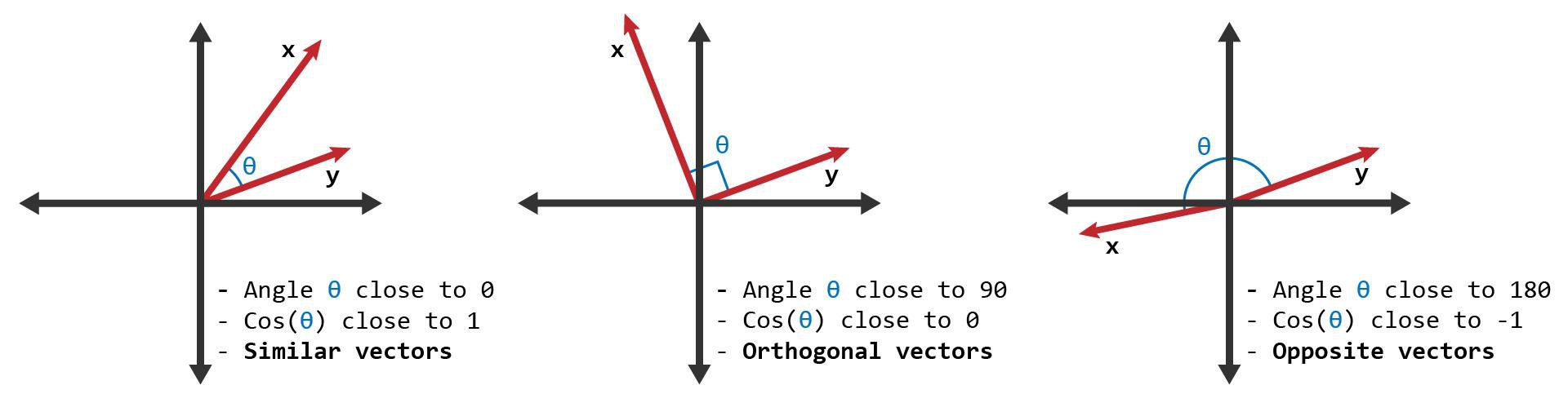
[Source: ScienceDirect]

Used Dataset

The dataset we’ll be using today is the Semantic Textual Similarity (STS) benchmark, one of the most varied and referenced datasets for this task. It comprises a selection of the English datasets used in the STS tasks organized in the context of semantic evaluation, adding up to over 5700 training instances.

Note that the dataset has other language variants, which recommends you use a multilingual BERT model, more on this via the official HuggingFace documentation.

Each instance is a pair of sentences, as well as their respective similarity score. However, a standard BERT model generates embeddings per token, and since our dataset comprises sentences, it would be not only more efficient but also scalable, to use sentence-level embeddings.

There are multiple ways to achieve this:

Taking the mean of the token embeddings generated by your standard BERT model.
Using the embedding of the classification token [CLS]
Using the max-over-time token-level embedding vectors (which means the element-wise maximum vector)

Model’s Architecture

For this tutorial, we will go for the first option among the ones mentioned above, which is the most used and recommended one. Luckily, it’s pretty simple to build our own special Sentence-level BERT by using the sentence-transformers library, this will result in the architecture illustrated below:

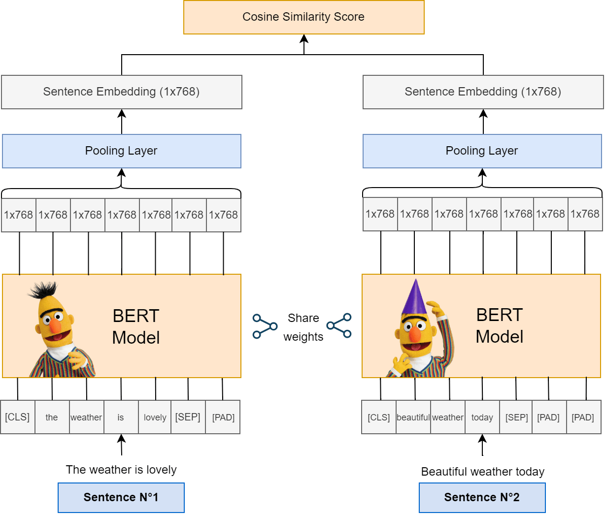
This architecture, which can be viewed as a Siamese-type model architecture (meaning that the BERT model will act as two identical sub-networks that share exactly the same weights and parameters), will allow the following:

Taking a pair of sentences (or any piece of text) as input.
Tokenization of the input (including the special tokens such as the classification token [CLS] and the separator token [SEP]).
Generation of 768-dimensional (the default dimension of BERT’s vector space) token-level embeddings for each sentence by the BERT model.
The Pooling Layer which, by default, performs a mean operation on the token embeddings, will allow for calculating of sentence-level embeddings.

Using the pair of sentence embeddings, a cosine similarity score is calculated to indicate how semantically similar they are.

Thanks to this architecture and to the similarity score feedback eventually received, the BERT model will learn to adjust its embeddings such that a pair of sentences with similar semantics will have similar vectors (speaking from a 768-dimensional vector space context).

Pretty simple, right?

Now as they say, ‘Talk is cheap, show me the code’. The full Colab notebook can be found here but make sure to stick around for more concise explanations.

Getting Started

We’ll start by installing the necessary packages, namely: transformers, sentence-transformers, and datasets in case you’re using Google Colab for the training. Otherwise, if you’re doing it locally, you’ll also need to install tqdm, pandas, numpy, and PyTorch (make sure to follow the official guide for a correct and compatible installation with your device)

If you’re not familiar with the package, Huggingface’s datasets will allow us to (you guessed it) load the dataset we’ll use for this tutorial:

$ pip install transformers sentence-transformers datasets

Then, we’ll import all the necessary packages as follows:

from datasets import load_dataset
from sentence_transformers import SentenceTransformer, models
from transformers import BertTokenizer
from transformers import get_linear_schedule_with_warmup
import torch
from torch.optim import AdamW
from torch.utils.data import DataLoader
from tqdm import tqdm
import time
import datetime
import random
import numpy as np
import pandas as pd

The next step would be to set the device we’ll train the model on, preferably a GPU. If it isn’t available, make sure you have set the correct runtime type on Google Colab (which can be accessed via Runtime > Change runtime type). Otherwise, we’ll proceed to set the famous device variable:

if torch.cuda.is_available():    
    device = torch.device("cuda")
    print(f'There are {torch.cuda.device_count()} GPU(s) available.')
    print('We will use the GPU:', torch.cuda.get_device_name(0))
else:
    print('No GPU available, using the CPU instead.')
    device = torch.device("cpu")

Loading and Previewing the Dataset

Next, we’ll easily load the STSB dataset from the Huggingface hub. Feel free to explore other datasets created especially for semantic textual similarity, or even upload and use your own dataset! More on this via Huggingface’s official datasets documentation.

# Load the English version of the STSB dataset
dataset = load_dataset("stsb_multi_mt", "en")
print(dataset)

The print() function allows us to check how our dataset looks from a high-surface level:

DatasetDict({
    train: Dataset({
        features: ['sentence1', 'sentence2', 'similarity_score'],
        num_rows: 5749
    })
    test: Dataset({
        features: ['sentence1', 'sentence2', 'similarity_score'],
        num_rows: 1379
    })
    dev: Dataset({
        features: ['sentence1', 'sentence2', 'similarity_score'],
        num_rows: 1500
    })
})

As you can see, the dataset comprises train, test, and dev (also known as validation) splits. Note that we’ll use both the train and dev sets during the training phase.

Let’s take a look at a sample from the STSB dataset, specifically the training split:

print("A sample from the STSB dataset's training split:")
print(dataset['train'][98])

Output:

{'sentence1': 'A man is slicing potatoes.', 'sentence2': 'A woman is peeling potato.', 'similarity_score': 2.200000047683716}

If you take a broader look at the dataset, you’ll see that the similarity scores have values ranging from 1 to 5. In order to align them with our cosine-similarity-based approach, we’ll normalize these scores such that they fall within a range of 0 to 1.

This means that the sample’s normalized similarity score is:

2.200000047683716/5.0 ≈ 0.44

Which clearly indicates that the pair of sentences cannot be considered semantically similar.

Preparing the Data

In order to provide our model with properly prepared data, we’ll define a custom data loader class named STSBDataset. A data loader class is necessary to efficiently load and prepare your data for training or inference in a Machine Learning setting. It provides functionality for loading data from a dataset, applying the necessary transformations or preprocessing steps, and batching the data for efficient processing.

But before looking into the details of it, let’s first define our tokenizer as we’ll be using it within our class:

# You can use larger variants of the model, here we're using the base model
tokenizer = BertTokenizer.from_pretrained('bert-base-uncased')

The STSBDataset class is then defined as follows:

class STSBDataset(torch.utils.data.Dataset):

    def __init__(self, dataset):
        # Normalize the similarity scores in the dataset
        similarity_scores = [i['similarity_score'] for i in dataset]
        self.normalized_similarity_scores = [i/5.0 for i in similarity_scores]
        self.first_sentences = [i['sentence1'] for i in dataset]
        self.second_sentences = [i['sentence2'] for i in dataset]
        self.concatenated_sentences = [[str(x), str(y)] for x,y in   zip(self.first_sentences, self.second_sentences)]

    def __len__(self):
        return len(self.concatenated_sentences)

    def get_batch_labels(self, idx):
        return torch.tensor(self.normalized_similarity_scores[idx])

    def get_batch_texts(self, idx):
        return tokenizer(self.concatenated_sentences[idx], padding='max_length', max_length=128, truncation=True, return_tensors="pt")

    def __getitem__(self, idx):
        batch_texts = self.get_batch_texts(idx)
        batch_y = self.get_batch_labels(idx)
        return batch_texts, batch_y


def collate_fn(texts):
    input_ids = texts['input_ids']
    attention_masks = texts['attention_mask']
    features = [{'input_ids': input_id, 'attention_mask': attention_mask}
                for input_id, attention_mask in zip(input_ids, attention_masks)]
    return features

As previously explained, the data loader class takes care of preparing the data from end to end, and that is by:

Retrieving the similarity scores from the dataset.
Dividing each score by 5.0 in order to normalize it.
Assembling the pairs of sentences into the concatenated_sentences attribute, for each row respectively.
Batching the pairs of sentences (after tokenizing each one at once) as well as the normalized similarity scores thanks to the get_batch_texts() and get_batch_labels() functions, respectively.

Note that the return_tensors="pt" argument of the tokenizer allows us to retrieve the batch’s PyTorch tensors and eventually move them to the GPU (also known as device). The tensors hold two types of information: input_ids which represent the tokens' identifying number within the tokenizer’s vocabulary, and attention_mask which allows the model to distinguish between the actual tokens and the added padding.

This is where the collate_fn() function comes in handy, its purpose is to provide a way to collate the individual preprocessed texts into batches that can be processed efficiently during training or inference. It ensures that the data loader returns batches in a format that can be directly fed into the model for processing. In our implementation, the function creates a list of feature dictionaries, where each dictionary represents a batch and contains the input_ids and attention_mask for that batch.

Defining the Model Class Based on BERT

Now that we’ve set the ground to prepare our data, let’s create the actual magician, the model.

As described by the architecture we defined above, our model has two main components: a BERT model, and a pooling layer which will allow us to retrieve the sentence embeddings. Instead of using them separately, we’ll hand them over to the SentenceTransformer by passing them as modules. This will tackle the processing more efficiently and will save us the burden of boilerplate code:

class BertForSTS(torch.nn.Module):

    def __init__(self):
        super(BertForSTS, self).__init__()
        self.bert = models.Transformer('bert-base-uncased', max_seq_length=128)
        self.pooling_layer = models.Pooling(self.bert.get_word_embedding_dimension())
        self.sts_bert = SentenceTransformer(modules=[self.bert, self.pooling_layer])

    def forward(self, input_data):
        output = self.sts_bert(input_data)['sentence_embedding']
        return output

By passing the pair of sentences to the model, it will generate their corresponding sentence embeddings and adjust its weights accordingly. The former can be easily retrieved through the sentence_embedding attribute of the model’s output.

Next, we’ll only have to create an instance of the model and move it to the device:

# Instantiate the model and move it to GPU
model = BertForSTS()
model.to(device)

Defining the Loss Function

Since our objective is to train a model to effectively differentiate between pairs of texts based on their semantic meaning. The desired outcome is for the model to learn to separate dissimilar text pairs by assigning them a large distance or dissimilarity score while keeping similar text pairs close together with a small distance or similarity score.

For this matter, we’ll use a loss function that’s very specific to our case: the Cosine similarity loss.

class CosineSimilarityLoss(torch.nn.Module):

    def __init__(self,  loss_fn=torch.nn.MSELoss(), transform_fn=torch.nn.Identity()):
        super(CosineSimilarityLoss, self).__init__()
        self.loss_fn = loss_fn
        self.transform_fn = transform_fn
        self.cos_similarity = torch.nn.CosineSimilarity(dim=1)

    def forward(self, inputs, labels):
        emb_1 = torch.stack([inp[0] for inp in inputs])
        emb_2 = torch.stack([inp[1] for inp in inputs])
        outputs = self.transform_fn(self.cos_similarity(emb_1, emb_2))
        return self.loss_fn(outputs, labels.squeeze())

Although customized, this loss is based on the Mean Squared Error (MSE) which is the standard metric for regression tasks such as STS. After retrieving the sentence pair embeddings, we’ll calculate the cosine similarity between them, and finally, the MSE will indicate how close the model is to the actual similarity value in our dataset.

Preparing the Training and Validation Data Splits

First, we’ll load the necessary splits through our data class:

train_ds = STSBDataset(dataset['train'])
val_ds = STSBDataset(dataset['dev'])

# Create a 90-10 train-validation split.
train_size = len(train_ds)
val_size = len(val_ds)

print('{:>5,} training samples'.format(train_size))
print('{:>5,} validation samples'.format(val_size))

The print() statement shows that we, in total, have 5,749 training samples and 1,500 validation samples.

batch_size = 8

train_dataloader = DataLoader(
            train_ds,  # The training samples.
            num_workers = 4,
            batch_size = batch_size, # Use this batch size.
            shuffle=True # Select samples randomly for each batch
        )

validation_dataloader = DataLoader(
            val_ds,
            num_workers = 4,
            batch_size = batch_size # Use the same batch size
        )

We’ll use a batch_size of 8, but feel free to experiment with different values. Avoid batch sizes that are too big, though, as it could potentially cause the model to diverge from the optimal set of weights.

Not to confuse it with our customized STSBDataset class, PyTorch’s DataLoader class takes care of further functionalities such as shuffling the data during the training, enabling multi-threaded data loading when requested by the user, and the overall integration of the training pipeline with Pytorch’s ecosystem.

Defining the Optimizer and Scheduler

For the optimizer, we’ll use AdamW with an initial learning rate of 1e-6. AdamW is an optimization algorithm commonly used for training deep neural networks. It’s an extension of the Adam optimizer that incorporates weight decay regularization to mitigate overfitting.

A scheduler refers to an object or component that dynamically adjusts the learning rate during the training process in order to improve its stability, and convergence and overall achieve better model performance. For this tutorial, we’ll use a linear learning rate scheduler.

If you want to learn more about them, this detailed article is well recommended.

optimizer = AdamW(model.parameters(),
                  lr = 1e-6)
epochs = 8
# Total number of training steps is [number of batches] x [number of epochs].
total_steps = len(train_dataloader) * epochs
scheduler = get_linear_schedule_with_warmup(optimizer,
                                            num_warmup_steps = 0,
                                            num_training_steps = total_steps)

We’ll train the model for 8 epochs, but you should definitely experiment with different numbers to find which value is best for your case, all while avoiding overfitting to the data.

Training the Model

It’s now time for the real deal, the actual training.

The training function might seem overwhelming at first glance, but it’s very simple to understand once you’re familiar with the different steps that the model goes through as the training goes on. Simply put, the training loop achieves the following:

Instantiation of the Cosine similarity loss.
Setting the seed for the sake of getting reproducible results each time.
For each batch in the training data, the model generates the corresponding sentence pair embeddings (for example, if your batch size is 16, the model generates 16 pairs of embeddings at once)
Calculation of the batch loss and adding it to the total training loss (eventually averaged)
Performing a backpropagation to update the model’s learned weights, and updating the optimizer as well as the scheduler.

Note that steps [2-5] are performed at each epoch, and the same concepts (minus the backpropagation and optimization/scheduling) are applied to the validation batches.

At the end of the training, we’ll have the final fine-tuned model as well as different statistics, most importantly the average training/validation loss of the model which reflects its performance.

def train():
  seed_val = 42
  criterion = CosineSimilarityLoss()
  criterion = criterion.cuda()
  random.seed(seed_val)
  torch.manual_seed(seed_val)
  # We'll store a number of quantities such as training and validation loss,
  # validation accuracy, and timings.
  training_stats = []
  total_t0 = time.time()
  for epoch_i in range(0, epochs):
      t0 = time.time()
      total_train_loss = 0
      model.train()
      # For each batch of training data...
      for train_data, train_label in tqdm(train_dataloader):
          train_data['input_ids'] = train_data['input_ids'].to(device)
          train_data['attention_mask'] = train_data['attention_mask'].to(device)
          train_data = collate_fn(train_data)
          model.zero_grad()
          output = [model(feature) for feature in train_data]
          loss = criterion(output, train_label.to(device))
          total_train_loss += loss.item()
          loss.backward()
          torch.nn.utils.clip_grad_norm_(model.parameters(), 1.0)
          optimizer.step()
          scheduler.step()

      # Calculate the average loss over all of the batches.
      avg_train_loss = total_train_loss / len(train_dataloader)            
      # Measure how long this epoch took.
      training_time = format_time(time.time() - t0)
      t0 = time.time()
      model.eval()
      total_eval_accuracy = 0
      total_eval_loss = 0
      nb_eval_steps = 0
      # Evaluate data for one epoch
      for val_data, val_label in tqdm(validation_dataloader):
          val_data['input_ids'] = val_data['input_ids'].to(device)
          val_data['attention_mask'] = val_data['attention_mask'].to(device)
          val_data = collate_fn(val_data)
          with torch.no_grad():        
              output = [model(feature) for feature in val_data]
          loss = criterion(output, val_label.to(device))
          total_eval_loss += loss.item()
      # Calculate the average loss over all of the batches.
      avg_val_loss = total_eval_loss / len(validation_dataloader)
      # Measure how long the validation run took.
      validation_time = format_time(time.time() - t0)
      # Record all statistics from this epoch.
      training_stats.append(
          {
              'epoch': epoch_i + 1,
              'Training Loss': avg_train_loss,
              'Valid. Loss': avg_val_loss,
              'Training Time': training_time,
              'Validation Time': validation_time
          }
      )
  return model, training_stats

# Launch the training
model, training_stats = train()

The following code allows us to visualize the statistics in a more organized manner:

# Create a DataFrame from our training statistics
df_stats = pd.DataFrame(data=training_stats)

# Use the 'epoch' as the row index
df_stats = df_stats.set_index('epoch')

# Display the table
df_stats

Output:

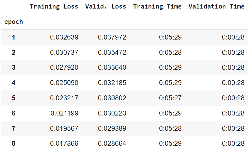
The statistics show that the validation Cosine similarity loss is continuously decreasing, which means that the model got more and more accurate at generating sentence embeddings in correspondence with semantic similarities of sentence pairs.

You can try to train the model for longer than 8 epochs for potentially better results.

Setting the Model for Inference

To evaluate our model’s performance, we’ll load the test split from our dataset and use a few examples from it to see how well the model represents sentence pairs in accordance with their semantics.

We’ll also define a predict_similarity() function that takes care of the necessary data preprocessing, as well as collecting the model’s semantic similarity prediction for a given pair of sentences:

# load the test set
test_dataset = load_dataset("stsb_multi_mt", name="en", split="test")

# Prepare the data
first_sent = [i['sentence1'] for i in test_dataset]
second_sent = [i['sentence2'] for i in test_dataset]
full_text = [[str(x), str(y)] for x,y in zip(first_sent, second_sent)]

model.eval()

def predict_similarity(sentence_pair):
  test_input = tokenizer(sentence_pair, padding='max_length', max_length = 128, truncation=True, return_tensors="pt").to(device)
  test_input['input_ids'] = test_input['input_ids']
  test_input['attention_mask'] = test_input['attention_mask']
  del test_input['token_type_ids']
  output = model(test_input)
  sim = torch.nn.functional.cosine_similarity(output[0], output[1], dim=0).item()
  return sim

Let’s try it out for a couple of sentence pairs:

Example 1:

example_1 = full_text[100]
print(f"Sentence 1: {example_1[0]}")
print(f"Sentence 2: {example_1[1]}")
print(f"Predicted similarity score: {round(predict_similarity(example_1), 2)}")

Sentence 1: A cat is walking around a house.
Sentence 2: A woman is peeling potato.

By calling the predict_similarity() function and rounding the result to two decimal places, we get the following output, rightfully so:

Predicted similarity score: 0.01

The sentence pair has no match in meaning, and the model correctly generated its embeddings as the similarity score is very close to 0.

Example 2:

example_2 = full_text[130]
print(f"Sentence 1: {example_2[0]}")
print(f"Sentence 2: {example_2[1]}")
print(f"Predicted similarity score: {round(predict_similarity(example_2), 2)}")

Sentence 1: Two men are playing football.
Sentence 2: Two men are practicing football.

Output

Predicted similarity score: 0.84

An opposite case is noticed in this second example, the two sentences are very close in meaning. Thus, a high similarity score is assigned to them.

Example 3:

example_3 = full_text[812]
print(f"Sentence 1: {example_3[0]}")
print(f"Sentence 2: {example_3[1]}")
print(f"Predicted similarity score: {round(predict_similarity(example_3), 2)}")

Sentence 1: It varies by the situation.
Sentence 2: This varies by institution.

Output:

Predicted similarity score: 0.6

For this last example, the sentences aren’t similar in meaning to a high extent, nor they don’t match in meaning. The model’s generated embeddings allowed for a similarity score of 0.6 which is well-suited for it.

Saving the Model

In order to save the model and, later on, load it for future inference and even exploit it for other tasks, you only have to define the saving path and call PyTorch’s .save() function while providing it with the model’s state dictionary (referred to as state_dict) which is simply a Python dictionary that stores the model’s parameters.

PATH = 'bert-sts.pt'
torch.save(model.state_dict(), PATH)

To load the model, you first have to create an instance of its class, then load it using PyTorch’s load_state_dict() function as well as the previously defined saving PATH:

# In order to load the model
# First, you have to create an instance of the model's class
# And use the saving path for the loading
# Don't forget to set the model to the evaluation state using .eval()
model = BertForSTS()
model.load_state_dict(torch.load(PATH))
model.eval()
# perform prediction as above...

More on saving and loading your PyTorch models can be found in their official documentation.

Conclusion

Measuring semantic textual similarity is one of the key tasks in NLP, and that is even further used in other, more complex tasks such as semantic search. This tutorial on fine-tuning BERT for semantic textual similarity has provided valuable insights into the process of adapting BERT, a powerful pre-trained language model, to this specific task.

We have tackled many important concepts for the whole training pipeline, namely: data preparation and preprocessing, creating a custom dataset class, as well as selecting an appropriate evaluation metric, such as the integration of Cosine similarity with mean squared error, to train and assess the model's performance.

All these steps, in addition to model/dataset loading, can be achieved in just a few lines of code thanks to the availability of various functionalities provided by the HuggingFace library as well as PyTorch. The best part of all this is that it’s fully customizable, meaning that you can experiment with your own data, different sets of hyperparameters, loss functions, you name it.

Hoping that this step-by-step tutorial has provided you with both a theoretical and technical deep-dive into the fine-tuning of Transformer-based language models such as BERT on a task that’s as essential to NLP as a semantic textual similarity.

You’re most welcome to expand your knowledge by trying out new tasks, models, and datasets!

Friendly reminder that the full code can be found as a Google Colab notebook, here.

Here are some other NLP tutorials:

References

Happy learning ♥

Why juggle between languages when you can convert? Check out our Code Converter. Try it out today!

View Full Code Create Code for Me

Sharing is caring!

Comment panel

Got a coding query or need some guidance before you comment? Check out this Python Code Assistant for expert advice and handy tips. It's like having a coding tutor right in your fingertips!