Step up your coding game with AI-powered Code Explainer. Get insights like never before!
Table of Contents
![]()
Introduction
One of the most fascinating recent advancements is the development of text-to-image generation models. These models have the ability to translate mere words into vivid, detailed visual representations, with numerous possibilities across vast sectors. However, anyone who has played with these models knows generating a perfect image from just a text prompt involves countless attempts and tweaks. But imagine if you could control what image is generated based on a pose or some edges or even depth maps, wouldn’t that be great? Lucky for us, we have ControlNet.
This article will give you a comprehensive understanding of ControlNet. We will dive into its in-depth operation and understand the math behind it. We will also learn to use it via Hugging Face and implement our ControlNet. This will give you a firsthand experience of its potential regardless of your prior experiences.
But before you dive into this article, it is highly recommended you check out our previous article on text-to-image diffusion models in case you’re not sure how diffusion models work.
ControlNet
ControlNet is a neural network model proposed by Lvmin Zhang and Maneesh Agrawala in the paper “Adding Conditional Control to Text-to-Image Diffusion Models'' to control pre-trained large diffusion models to support additional input conditions (i.e., besides text prompt). ControlNet can learn the task-specific conditions in an end-to-end manner with less than 50,000 samples, making training as fast as fine-tuning a diffusion model.
ControlNet mitigates several problems of the existing stable diffusion models that need to be used for specific tasks:
- In task-specific domains, available data is not as large as the one used frequently in the more general image-text domain.
- Training the large diffusion models requires large clusters of high-end GPUs which isn’t always feasible. This necessitates the use of pre-trained weights through either fine-tuning, transfer learning, or some other technique.
- Constraining diffusion models without handcrafted rules is not always feasible, requiring some kind of automatic interpretation of raw inputs.
ControlNet takes care of all these and has been implemented for several different kinds of conditioning:
| Canny Edge |
These are the edges detected using the Canny Edge Detection algorithm used for detecting a wide range of edges. It involves the removal of noise in the input image using a Gaussian filter, calculation of the intensity gradient of the image, non-maximum suppression to thin out edges, and hysteresis thresholding to determine the edges. This conditioning is good at detecting edges while suppressing noise. It is also more suitable when the edges are continuous. |
| Hough Line |
These are detected using the more recent deep Hough transform instead of the traditional Hough transform algorithm. Hough lines are mainly used mainly in computer vision to detect straight lines making them particularly helpful in shape recognition. The authors create their dataset from the Places2 dataset by using BLIP to generate captions. Check this tutorial to learn more about BLIP. Due to its straight-line detection nature, this conditioning is particularly good at generating wireframes for images (like for interior design). It is also helpful when trying to detect lines that are broken or distorted. |
| HED Boundary |
HED or “Holistically-Nested Edge Detection”, is another edge detection algorithm using fully convolutional neural networks. This conditioning is good at preserving many details from the input images. This makes it suitable for recoloring and styling images. |
| User Sketching | This is used to generate images from user sketches or scribbles. |
| Human Pose |
This uses the open-source Openpose model to detect the human pose in a reference image and constrains the ControlNet model on the same. This conditioning is particularly good for generating certain poses. |
| Semantic Segmentation | Semantic segmentation labels each pixel of an image with a corresponding class. This is a typical computer vision task and has several different approaches. The authors however create their dataset from the COCO and the ADE20K dataset (which consists of images and their semantic segmentations labeled) by using BLIP for generating captions. |
| Depth |
Depth images contain information about the distance of objects from the camera. This is a popular task in computer vision and is also used in it to provide additional information about 3D scenes. This conditioning is quite good in natural scenes like landscapes where different objects are present at different depths. |
| Normal Maps |
Normal maps are a type of bump map representing different surface details like bumps, grooves, and scratches to a model. Each pixel in the normal map contains information about the direction of the surface normal at that point on the model. The authors use the DIODE dataset captioned by BLIP to train their ControlNet model. These are useful when trying to add surface-level details. |
| Cartoon Line Drawings | This model is trained by using a cartoon line drawing extracting method on cartoon illustrations from the internet. |
Examples of several conditioned images are available here.
Working
ControlNet works by manipulating the input conditions of the neural network blocks in order to control the behavior of the entire neural network. It does this by cloning the diffusion model into a locked copy and a trainable copy.
While training only the trainable copy of the model is updated. The locked copy preserves the capabilities of the network learned from the general image-text datasets. These production-ready weights also help robustly train datasets at different scales.
The trainable copy is trained on the task-specific dataset to learn the conditional controls. It interacts with the locked copy to inject the input image constraints into the overall model. The authors who proposed ControlNet also demonstrate that training the model on a personal computer (one Nvidia RTX 2090Ti) is competitive with commercial models trained on large clusters with terabytes of GPU memory.
These two copies are connected via a special type of convolution layer called zero convolution. It is a 1x1 convolution layer initialized with zeros. The weights of the zero convolution layer progressively update from zero to the optimized values.
How ControlNet Modifies a Single Neural Network Block
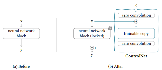
Let’s for a moment assume, we don’t have a ControlNet as depicted by the figure on the left. The neural network block can then be thought of as a function F that takes an input feature map x and outputs another feature map y such that y = F(x; θ) where θ (and its subscripts as used later) represent the neural network weights.
Now let’s add a ControlNet module to this block as depicted by the figure on the right. Suppose the output of a zero convolution is represented by Z and the external conditional vector is represented by c. Then the output after the first zero convolution is Z(c; θ_z1) which is then added to the input x giving us a new input: x + Z(c; θ_z1) for the trainable copy. The output of this trainable copy can be represented as F(x + Z(c; θ_z1); θ_c). This output is then passed to a zero convolution layer and the final output from the ControlNet is thus Z(F(x + Z(c; θ); θ_c); θ_z2).
Finally, we do an element-wise addition of the outputs of our locked copy and the trainable copy to get the following final output:
y_c = F(x; θ) + Z(F(x + Z(c; θ); θ_c); θ_z2)
This mathematical point of view we just discussed illustrates how the input to the trainable copy is modified to adjust for our image constraints.
Since the zero convolution layers are initialized with zeros, any output in the beginning regardless of the input would be a feature map full of zeros. Essentially, we have the second term of the equation representing y_c as zero implying y_c = F(x; θ) in the first training step. Intuitively this means all the inputs and outputs of both the trainable and locked copies of neural network blocks are consistent with what they would be if the ControlNet does not exist. In other words, the ControlNet model does not influence the deep neural features in the very first round.
However, this will not be the case in further training rounds when the zero convolution layer weights are updated to become non-zero. The capability, functionality, and result quality of any neural network block is perfectly preserved and any further optimization will become as fast as fine-tuning in comparison to training those layers from scratch.
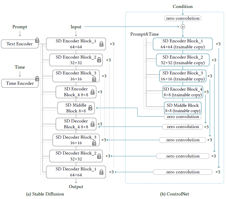
How ControlNet Modifies the Entire Image Diffusion Model
The stable diffusion model is a U-Net with an encoder, a skip-connected decoder, and a middle block. As shown in the diagram, both the encoder and the decoder have 12 blocks each (3 64x64 blocks, 3 32x32 blocks, and so on). The diffusion models also work by converting the original 512x512 images into the smaller 64x64 latent images for stabilized learning. This makes it necessary to convert the image-based conditions to the 64x64 size so as to match the convolution size. To achieve this, a tiny network of four convolution layers with 4x4 kernels and 2x2 strides is used.
Training the Model
Since connecting ControlNet does not require training the locked parameters, during training no gradient computation for them is required. This speeds up the training process and saves GPU memory, as half of the gradient computation on the original model can be avoided.
Using a ControlNet also modifies the learning objective. Instead of now predicting noise from just the noisy image, the timestep, and the text prompt, we also have task-specific conditions (the conditional input image).
During training, we can also randomly replace 50% of the text prompts with empty strings (as done by the original authors) to facilitate ControlNet’s ability to recognize semantic contents from input condition maps (which makes sense because the prompt is not visible and the only clue is in the conditional image).
Code
Now that we understand how it works in theory, let’s get our hands dirty with some code on Google Colab. Before you begin, make sure you have GPU enabled. To do so, go to Runtime, click change runtime type, and select GPU from the hardware accelerator option.
Let’s begin by installing the 🤗 Transformers library and the necessary libraries required to speed up the inference:
$ pip install -qU xformers diffusers transformers accelerateLet’s also install the following libraries required by the ControlNet to preprocess the reference images to generate the images stable diffusion would be conditioned on:
$ pip install -qU  controlnet_aux
$ pip install opencv-contrib-python
Open-pose
Let’s begin with the Open Pose ControlNet model and import the following required libraries:
from PIL import Image
from diffusers import StableDiffusionControlNetPipeline, ControlNetModel, UniPCMultistepScheduler
import torch
from controlnet_aux import OpenposeDetector
from diffusers.utils import load_image
from tqdm import tqdm
from torch import autocast
We will now load all the required stuff like the pose detection model, the pre-trained ControlNet model, the diffusion pipeline that incorporates ControlNet, and the scheduler used by this pipeline:
# load the openpose model
openpose = OpenposeDetector.from_pretrained('lllyasviel/ControlNet')
# load the controlnet for openpose
controlnet = ControlNetModel.from_pretrained("lllyasviel/sd-controlnet-openpose", torch_dtype=torch.float16)
# define stable diffusion pipeline with controlnet
pipe = StableDiffusionControlNetPipeline.from_pretrained("runwayml/stable-diffusion-v1-5", controlnet=controlnet, safety_checker=None, torch_dtype=torch.float16)
pipe.scheduler = UniPCMultistepScheduler.from_config(pipe.scheduler.config)
An important thing to notice here is how we pass the controlnet to the pipeline we defined.
Also, notice we use the UniPCMultiStepScheduler. This is a scheduler designed for fast sampling of diffusion models and is designed specifically for the UniPC framework which itself is a training-free framework supporting pixel-space as well as latent space and is model-agnostic! We will be using this scheduler in all the different variants of ControlNet as explored further in the article.
Let’s now enable efficient computation of the attention mechanism using the xformers library which we deliberately installed in the beginning:
# enable efficient implementations using xformers for faster inference
pipe.enable_xformers_memory_efficient_attention()
pipe.enable_model_cpu_offload()
Now we need an input image, which can be loaded as follows:
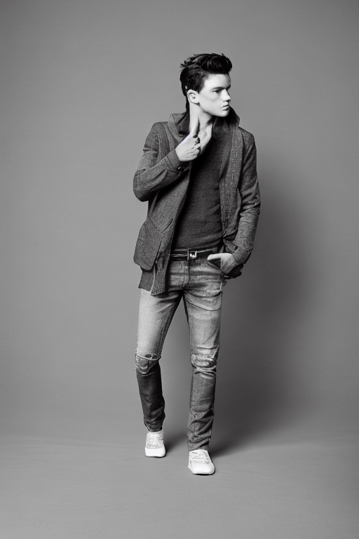
image_input = load_image("https://cdn.pixabay.com/photo/2016/05/17/22/19/fashion-1399344_640.jpg")
image_input
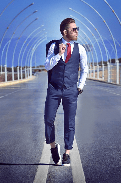
We will take this image of the man, and try to generate another fashion model in the same pose. But first, we need to get his pose from the picture. Lucky for us, the openpose model we loaded does it for us in just a single line:
image_pose = openpose(image_input)
image_pose
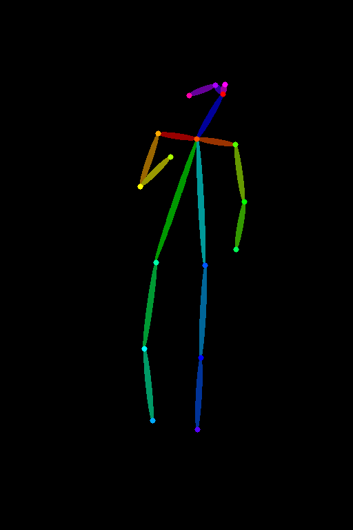
Notice how this stick figure kind of structure captures different body parts of the pose. Different joints are drawn as circles and these are called keypoints which is exactly what the pose detection models predict. The different color lines represent limbs, for instance, the neck is dark blue, the torso is lime green, and so on.
The best part is that you can also draw this stick figure yourself if you follow this color scheme and generate images using that!
Finally, let’s now give a prompt, and the previously detected pose to our pipeline to generate an image. In this tutorial, we will use 20 inference steps for all the examples, however, you can use even more and experiment with which one suits you the best:
image_output = pipe("A professional photograph of a male fashion model", image_pose, num_inference_steps=20).images[0]
image_output
Look at that! Isn’t this cool?
Canny
We just saw how to generate images using OpenPose. Let’s now see what the Canny version does. Just like before we will import the required libraries:
import cv2
from PIL import Image
from diffusers import StableDiffusionControlNetPipeline, ControlNetModel, UniPCMultistepScheduler
import torch
import numpy as np
from diffusers.utils import load_image
Then we will load different models and enable efficient computation:
# load the controlnet model for canny edge detection
controlnet = ControlNetModel.from_pretrained("lllyasviel/sd-controlnet-canny", torch_dtype=torch.float16)
# load the stable diffusion pipeline with controlnet
pipe = StableDiffusionControlNetPipeline.from_pretrained("runwayml/stable-diffusion-v1-5", controlnet=controlnet, safety_checker=None, torch_dtype=torch.float16)
pipe.scheduler = UniPCMultistepScheduler.from_config(pipe.scheduler.config)
# enable efficient implementations using xformers for faster inference
pipe.enable_xformers_memory_efficient_attention()
pipe.enable_model_cpu_offload()
We now load a new image to demonstrate this canny variant of ControlNet better. We will try to generate a new colorful bird:
image_input = load_image("https://cdn.pixabay.com/photo/2023/06/03/16/05/spotted-laughingtrush-8037974_640.png")
image_input = np.array(image_input)
Image.fromarray(image_input)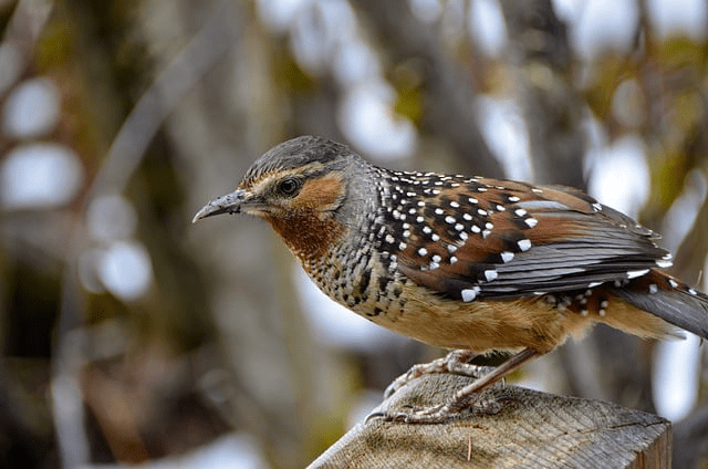
To do the canny edge detection, we specify the low and high threshold parameters for the Canny Edge Detection algorithm implemented in the OpenCV library. We then convert the output to the PIL image format:
# define parameters from canny edge detection
low_threshold = 100
high_threshold = 200
# do canny edge detection
image_canny = cv2.Canny(image_input, low_threshold, high_threshold)
# convert to PIL image format
image_canny = image_canny[:, :, None]
image_canny = np.concatenate([image_canny, image_canny, image_canny], axis=2)
image_canny = Image.fromarray(image_canny)
image_canny
Related: How to Perform Edge Detection in Python using OpenCV.
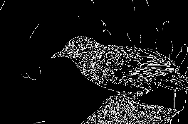
Notice how we have so many crisp white edges. Let’s now make a beautiful colorful bird from these edges:
image_output = pipe("a cute blue bird with colorful aesthetic feathers", image_canny, num_inference_steps=20).images[0]
image_output
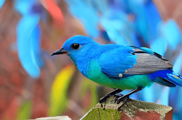
The bird we just generated looks so adorable!
Depth
Following the same process as before we will load all the required libraries and models:
from transformers import pipeline
from diffusers import StableDiffusionControlNetPipeline, ControlNetModel, UniPCMultistepScheduler
from PIL import Image
import numpy as np
import torch
from diffusers.utils import load_image

# load the depth estimator model
depth_estimator = pipeline('depth-estimation')
# load the controlnet model for depth estimation
controlnet = ControlNetModel.from_pretrained("lllyasviel/sd-controlnet-depth", torch_dtype=torch.float16)
# load the stable diffusion pipeline with controlnet
pipe = StableDiffusionControlNetPipeline.from_pretrained("runwayml/stable-diffusion-v1-5", controlnet=controlnet, safety_checker=None, torch_dtype=torch.float16)
pipe.scheduler = UniPCMultistepScheduler.from_config(pipe.scheduler.config)
# enable efficient implementations using xformers for faster inference
pipe.enable_xformers_memory_efficient_attention()
pipe.enable_model_cpu_offload()
We now load a sample image from the ControlNet Hugging Face repository:
image_input = load_image("https://huggingface.co/lllyasviel/sd-controlnet-depth/resolve/main/images/stormtrooper.png")
image_input
We now pass our downloaded image to the depth estimator model and convert it to PIL image format to get the image depths:
# get depth estimates
image_depth = depth_estimator(image_input)['depth']
# convert to PIL image format
image_depth = np.array(image_depth)
image_depth = image_depth[:, :, None]
image_depth = np.concatenate([image_depth, image_depth, image_depth], axis=2)
image_depth = Image.fromarray(image_depth)
image_depth
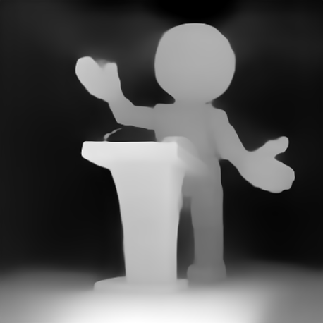
Notice how the robot and the stand are not completely black and the stand’s depth image is brighter than that of the robot. The nearer the object, the lighter its depth map representation.
Learn also: Image to Image Generation with Stable Diffusion in Python.
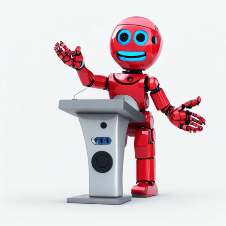
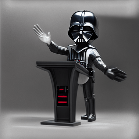
Let’s now make an image of Darth Vader giving the lecture as follows:
image_output = pipe("A realistic, aesthetic portrait style photograph of Darth Vader giving lecture, 8k, unreal engine", image_depth, num_inference_steps=20).images[0]
image_output
Normal
Let’s now try ControlNet on normal images. We need to follow the same procedure as before, so let’s skip directly to loading and processing the image:
from PIL import Image
from transformers import pipeline
import numpy as np
import cv2
from diffusers import StableDiffusionControlNetPipeline, ControlNetModel, UniPCMultistepScheduler
import torch
from diffusers.utils import load_image
# load the Dense Prediction Transformer (DPT) model for getting normal maps
depth_estimator = pipeline("depth-estimation", model ="Intel/dpt-hybrid-midas")
# load the controlnet model for normal maps
controlnet = ControlNetModel.from_pretrained(
"fusing/stable-diffusion-v1-5-controlnet-normal", torch_dtype=torch.float16
)
# load the stable diffusion pipeline with controlnet
pipe = StableDiffusionControlNetPipeline.from_pretrained(
"runwayml/stable-diffusion-v1-5", controlnet=controlnet, safety_checker=None, torch_dtype=torch.float16
)
pipe.scheduler = UniPCMultistepScheduler.from_config(pipe.scheduler.config)
# enable efficient implementations using xformers for faster inference
pipe.enable_xformers_memory_efficient_attention()
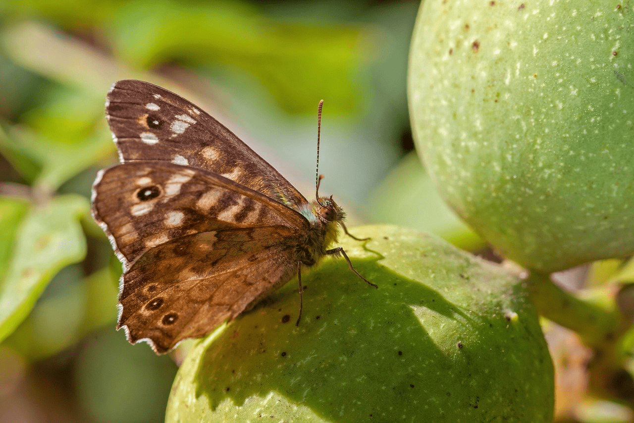
pipe.enable_model_cpu_offload()Here we load an image of a butterfly. Let’s turn those green fruits into apples:
image_input = load_image("https://cdn.pixabay.com/photo/2023/06/07/13/02/butterfly-8047187_1280.jpg")
image_input
We will first estimate the depths using Intel’s DPT Hybrid Midas model. DPT stands for Dense Prediction Transformer and is used for monocular depth prediction or just depth estimation. We normalize these depth maps and pass them through the Sobel operators from cv2. These outputs are then thresholded to separate the background from the objects in the foreground and are concatenated as done in the code:
# do all the preprocessing to get the normal image
image = depth_estimator(image_input)['predicted_depth'][0]
image = image.numpy()

image_depth = image.copy()
image_depth -= np.min(image_depth)
image_depth /= np.max(image_depth)

bg_threhold = 0.4

x = cv2.Sobel(image, cv2.CV_32F, 1, 0, ksize=3)
x[image_depth < bg_threhold] = 0

y = cv2.Sobel(image, cv2.CV_32F, 0, 1, ksize=3)
y[image_depth < bg_threhold] = 0
z = np.ones_like(x) * np.pi * 2.0
image = np.stack([x, y, z], axis=2)
image /= np.sum(image ** 2.0, axis=2, keepdims=True) ** 0.5
image = (image * 127.5 + 127.5).clip(0, 255).astype(np.uint8)
image_normal = Image.fromarray(image)
image_normal
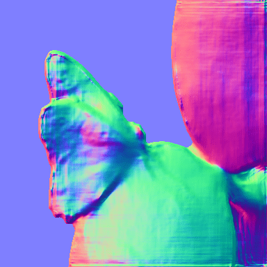
Notice the different RGB colors and how the fruit on the top is red and the one on the bottom is green. The normal maps display the surface normals of the image where the red, green, and blue colors represent the X, Y, and Z coordinates of the surface normals. Since the fruits in the original image had different orientations (they were almost perpendicular), their surface normals are also different and hence the different colors!
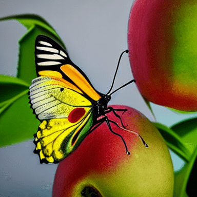
Let’s convert it into a beautiful butterfly sitting on apples:
image_output = pipe("A colorful butterfly sitting on apples", image_normal, num_inference_steps=20).images[0]
image_output
While ControlNet allows us to use reference images to generate more specific images, we can use it to generate pretty much anything and the model will try its best to fit our prompt with the input conditional image. For instance, if we instead ask the diffusion model to make a design, this is what we get:
image_output = pipe("A beautiful design", image_normal, num_inference_steps=20).images[0]
image_output
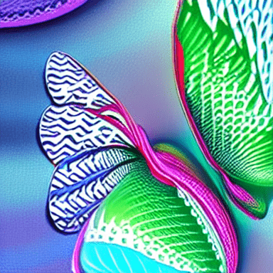
This pattern resembles our original image so much! People are using tricks like these with combinations of different models and parameter settings to generate amazing new stuff like “QR code art” as shown in this tweet. Surprisingly, most of these QR codes are scannable and work!
Semantic Segmentation
Though there are more versions of ControlNet, this will be the last one we explore in this article. If you have been diligently following the tutorial, you’ll face no problem trying the remaining ones yourselves.
After going through the codes below, let’s quickly skip to the processing part:
from transformers import AutoImageProcessor, UperNetForSemanticSegmentation
from PIL import Image
import numpy as np
import torch
from diffusers import StableDiffusionControlNetPipeline, ControlNetModel, UniPCMultistepScheduler
from diffusers.utils import load_image

# load the image processor and the model for doing segmentation
image_processor = AutoImageProcessor.from_pretrained("openmmlab/upernet-convnext-small")
image_segmentor = UperNetForSemanticSegmentation.from_pretrained("openmmlab/upernet-convnext-small")
# load the controlnet model for semantic segmentation
controlnet = ControlNetModel.from_pretrained("lllyasviel/sd-controlnet-seg", torch_dtype=torch.float16)
# load the stable diffusion pipeline with controlnet
pipe = StableDiffusionControlNetPipeline.from_pretrained("runwayml/stable-diffusion-v1-5", controlnet=controlnet, safety_checker=None, torch_dtype=torch.float16)
pipe.scheduler = UniPCMultistepScheduler.from_config(pipe.scheduler.config)
# enable efficient implementations using xformers for faster inference
pipe.enable_xformers_memory_efficient_attention()
pipe.enable_model_cpu_offload()
Besides loading everything we need, we also define a color palette to be used for the segmentation maps:
# define color palette that is used by the semantic segmentation models
palette = np.asarray([
    [0, 0, 0],
    [120, 120, 120],
    [180, 120, 120],
    ...
    [25, 194, 194],
    [102, 255, 0],
    [92, 0, 255],
])
Note: The palette consists of many colors, and hence has been shortened to keep the article concise. You can see the entire palette in the code file.
We now load our image:
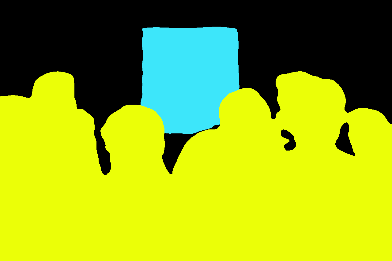
image_input = load_image("https://cdn.pixabay.com/photo/2023/02/24/07/14/crowd-7810353_1280.jpg")
image_input
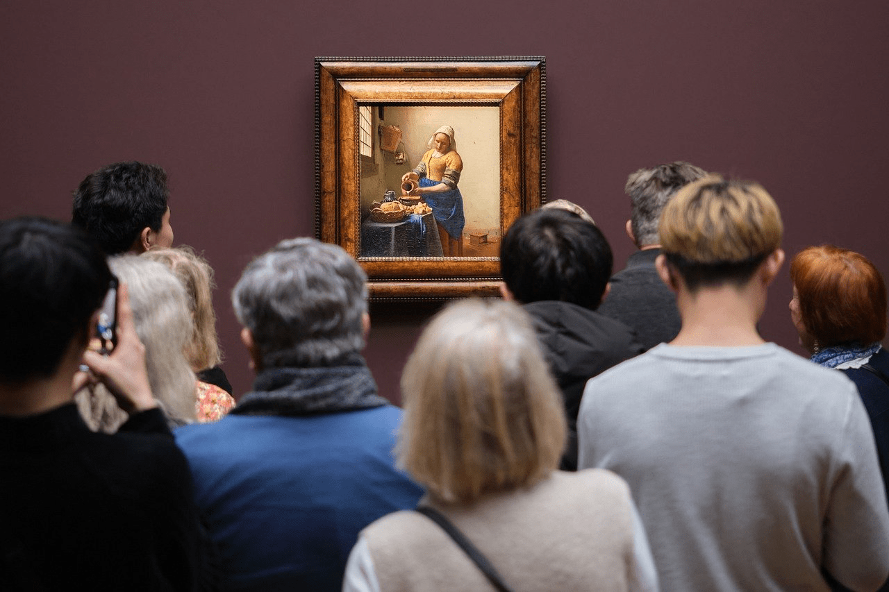
We will convert this image into different segment maps, using the upernet-convnext model as loaded before, and will utilize the predefined methods for preprocessing and postprocessing. Finally, we’ll add colors to different labels from our color palette and convert it into the PIL image format:
# get the pixel values
pixel_values = image_processor(image_input, return_tensors="pt").pixel_values
# do semantic segmentation
with torch.no_grad():
  outputs = image_segmentor(pixel_values)
# post process the semantic segmentation
seg = image_processor.post_process_semantic_segmentation(outputs, target_sizes=[image_input.size[::-1]])[0]
# add colors to the different identified classes
color_seg = np.zeros((seg.shape[0], seg.shape[1], 3), dtype=np.uint8) # height, width, 3
for label, color in enumerate(palette):
    color_seg[seg == label, :] = color
# convert into PIL image format
color_seg = color_seg.astype(np.uint8)
image_seg = Image.fromarray(color_seg)
image_seg
Related: How to Perform Image Segmentation using Transformers in Python
Notice how all the people were given the same yellow color. This is because it’s semantic segmentation (some other kinds of segmentation also give different colors to different instances of the same class). Now let’s convert this into a new AI-generated image:
image_output = pipe("A crowd of people staring at a glorious painting", image_seg, num_inference_steps=20).images[0]
image_output
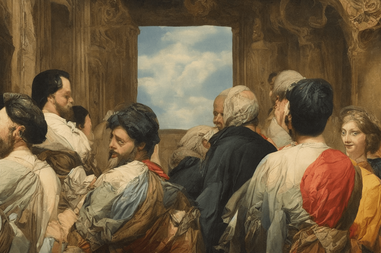
The image looks a little creepy but it does follow the “semantics” of the image. We can tune different models, or use ControlNet with a different base model to get a more aesthetic-looking image.
Custom Implementation of ControlNet
We have been through so many variations of ControlNet so we’ll now understand how to implement this framework ourselves.
Let’s begin with creating our custom ControlNet pipeline which takes several important components to be initialized. The various components can be seen in the code below:
class ControlNetDiffusionPipelineCustom:
    """custom implementation of the ControlNet Diffusion Pipeline"""
    def __init__(self, vae, tokenizer, text_encoder,
                 unet, controller, scheduler, image_processor,
                 control_image_processor):
        self.vae = vae
        self.tokenizer = tokenizer
        self.text_encoder = text_encoder
        self.unet = unet
        self.scheduler = scheduler
        self.controlnet = controlnet
        self.image_processor = image_processor
        self.control_image_processor = control_image_processor
        self.device = 'cuda' if torch.cuda.is_available() else 'cpu'
We will now define methods to get text embeddings and prompt embeddings:
    def get_text_embeds(self, text):
        """returns embeddings for the given `text`"""
        # tokenize the text
        text_input = self.tokenizer(text,
                                    padding='max_length',
                                    max_length=tokenizer.model_max_length,
                                    truncation=True,
                                    return_tensors='pt')
        # embed the text
        with torch.no_grad():
            text_embeds = self.text_encoder(text_input.input_ids.to(self.device))[0]
        return text_embeds

    def get_prompt_embeds(self, prompt):
        """returns prompt embeddings based on classifier free guidance"""
        if isinstance(prompt, str):
            prompt = [prompt]
        # get conditional prompt embeddings
        cond_embeds = self.get_text_embeds(prompt)
        # get unconditional prompt embeddings
        uncond_embeds = self.get_text_embeds([''] * len(prompt))
        # concatenate the above 2 embeds
        prompt_embeds = torch.cat([uncond_embeds, cond_embeds])
        return prompt_embeds
The get_prompt_embeds() method utilizes the get_text_embeds() method to generate embeddings for doing classifier-free guidance.
We now define a method to post-process images for us. This method takes the raw output by the VAE and converts it to the PIL image format:
    def transform_image(self, image):
        """convert image from pytorch tensor to PIL format"""
        image = self.image_processor.postprocess(image, output_type='pil')
        return image
Next, we define a method that samples a random image latent of appropriate shape as follows and scales it for the scheduler:
    def get_initial_latents(self, height, width, num_channels_latents, batch_size):
        """returns noise latent tensor of relevant shape scaled by the scheduler"""
        image_latents = torch.randn((batch_size,
                                   num_channels_latents,
                                   height // 8,
                                   width // 8)).to(self.device)
        # scale the initial noise by the standard deviation required by the scheduler
        image_latents = image_latents * self.scheduler.init_noise_sigma
        return image_latents
Next, we come to the most important method which will denoise the latents to create the actual image:
    def denoise_latents(self, prompt_embeds, controlnet_image,
                        timesteps, latents, guidance_scale=7.5):
        """denoises latents from noisy latent to a meaningful latent as conditioned by controlnet"""
        # use autocast for automatic mixed precision (AMP) inference
        with autocast('cuda'):
            for i, t in tqdm(enumerate(timesteps)):
                # duplicate image latents to do classifier free guidance
                latent_model_input = torch.cat([latents] * 2)
                latent_model_input = self.scheduler.scale_model_input(latent_model_input, t)
                control_model_input = latents
                controlnet_prompt_embeds = prompt_embeds
                # get output from the control net blocks
                down_block_res_samples, mid_block_res_sample = self.controlnet(
                    control_model_input,
                    t,
                    encoder_hidden_states=controlnet_prompt_embeds,
                    controlnet_cond=controlnet_image,
                    conditioning_scale=1.0,
                    return_dict=False,
                )
                # predict noise residuals
                with torch.no_grad():
                    noise_pred = self.unet(
                        latent_model_input,
                        t,
                        encoder_hidden_states=prompt_embeds,
                        down_block_additional_residuals=down_block_res_samples,
                        mid_block_additional_residual=mid_block_res_sample,
                    )['sample']
                # separate predictions for unconditional and conditional outputs
                noise_pred_uncond, noise_pred_text = noise_pred.chunk(2)
                # perform guidance
                noise_pred = noise_pred_uncond + guidance_scale * (noise_pred_text - noise_pred_uncond)
                # remove the noise from the current sample i.e. go from x_t to x_{t-1}
                latents = self.scheduler.step(noise_pred, t, latents)['prev_sample']
        return latents
We use autocasting to use mixed precision which lets us do inference faster. During each timestep, we duplicate the image latents because we’re doing classifier-free guidance, then make the input latents and prompt embeds for ControlNet and pass it to the ControlNet model and get the outputs for the downsampling block and the middle block. We use these outputs and pass them as additional residuals to our U-Net which automatically adds these residuals to the down blocks (the middle and the decoder blocks) in the U-Net as we previously discussed in the ControlNet diagram. This gives us the noise predictions for the conditional and unconditional inputs on which we do classifier-free guidance to get the final noise predictions. This predicted noise is removed from the latents through the scheduler.step() method.
Now all there’s left is to define a helper method for handling preprocessing:
    def prepare_controlnet_image(self, image, height, width):
        """preprocesses the controlnet image"""
        # process the image
        image = self.control_image_processor.preprocess(image, height, width).to(dtype=torch.float32)
        # send image to CUDA
        image = image.to(self.device)
        # repeat the image for classifier free guidance
        image = torch.cat([image] * 2)
        return image
We're utilizing the control_image_processor component to preprocess.
Finally, we’ll utilize and combine all the helper methods we just wrote into a single ready-to-use method below. It should be easy for you to follow the code as we have already covered what all the previously defined methods do:
    def __call__(self, prompt, image, num_inference_steps=20,
                 guidance_scale=7.5, height=512, width=512):
        """generates new image based on the `prompt` and the `image`"""
        # encode input prompt
        prompt_embeds = self.get_prompt_embeds(prompt)
        # prepare image for controlnet
        controlnet_image = self.prepare_controlnet_image(image, height, width)
        height, width = controlnet_image.shape[-2:]
        # prepare timesteps
        self.scheduler.set_timesteps(num_inference_steps)
        timesteps = self.scheduler.timesteps
        # prepare the initial image in the latent space (noise on which we will do reverse diffusion)
        num_channels_latents = self.unet.config.in_channels
        batch_size = prompt_embeds.shape[0] // 2
        latents = self.get_initial_latents(height, width, num_channels_latents, batch_size)
        # denoise latents
        latents = self.denoise_latents(prompt_embeds,
                                       controlnet_image,
                                       timesteps,
                                       latents,
                                       guidance_scale)
        # decode latents to get the image into pixel space
        latents = latents.to(torch.float16) # change dtype of latents since
        image = self.vae.decode(latents / self.vae.config.scaling_factor, return_dict=False)[0]
        # convert to PIL Image format
        image = image.detach() # detach to remove any computed gradients
        image = self.transform_image(image)
        return image
An important thing to notice is before converting the output of the VAE’s decoder into the PIL image (i.e., transform_image() method) we need to remove any gradients that might be associated with it. This is because PyTorch doesn’t allow tensors with gradients to be converted to the intermediary numpy arrays.
Now that we’re done coding our custom pipeline, let’s test it. We will first need all the components for our pipeline which can be extracted from any of the Hugging Face pipelines we used earlier. We are going to continue with the OpenPose variant and use the same example image:
# We can get all the components from the ControlNet Diffusion Pipeline (the one implemented by Hugging Face as well)
vae = pipe.vae
tokenizer = pipe.tokenizer
text_encoder = pipe.text_encoder
unet = pipe.unet
controlnet = pipe.controlnet
scheduler = pipe.scheduler
image_processor = pipe.image_processor
control_image_processor = pipe.control_image_processor
Next, we create an instance of our pipeline.
custom_pipe = ControlNetDiffusionPipelineCustom(vae, tokenizer, text_encoder, unet, controlnet, scheduler, image_processor, control_image_processor)And finally, we give it a prompt and the conditional image and we get the following output:
# sample image 1
images_custom = custom_pipe("a fashion model wearing a beautiful dress", image_pose, num_inference_steps=20)
images_custom[0]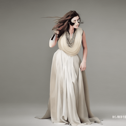
Hurray, our custom pipeline works! Let’s now create something else:
# sample image with a different prompt
images_custom = custom_pipe("A professional ice skater wearing a dark blue jacket around sunset, realistic, UHD", image_pose, num_inference_steps=20)
images_custom[0]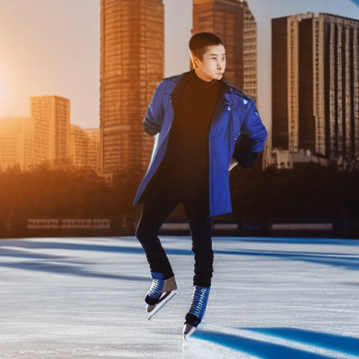
Anyways, that was a lot to cover, but at least now we know ControlNets in so much depth.
Conclusion
In this in-depth article, we learned how to control the image that is generated by text-to-image models using ControlNet. We also saw how ControlNet works both mathematically and in practice and explored its different variants. Finally, we used ControlNet ourselves using the HuggingFace Transformers and Diffusers libraries and also implemented it on our own.
You now have all the information you need to make and control your beautiful image generations. Get the complete code here.
Learn also: Image to Image Generation with Stable Diffusion in Python
Happy learning ♥
![]()
References
- Hugging Face space containing various ControlNet models:
- The original paper
- ControlNet implementation in Diffusers library:
Save time and energy with our Python Code Generator. Why start from scratch when you can generate? Give it a try!
View Full Code Improve My Code


Got a coding query or need some guidance before you comment? Check out this Python Code Assistant for expert advice and handy tips. It's like having a coding tutor right in your fingertips!